The Probabilistic Logic of Normal Distribution

The normal distribution is perhaps the most significant concept in modern statistics, serving as the foundational model for understanding how data behaves in the natural and social worlds. When individuals ask "what is normal distribution", they are often seeking an explanation for why so many diverse phenomena—from the heights of redwood trees to the errors in astronomical measurements—cluster around a central average in a predictable, symmetrical pattern. Often referred to as the bell curve due to its distinctive shape, this mathematical construct allows researchers to move beyond simple observation into the realm of precise prediction and inference. By defining the mathematical relationship between the mean and the spread of data, the normal distribution provides a universal language for quantifying uncertainty and identifying what qualifies as "expected" versus "extreme."

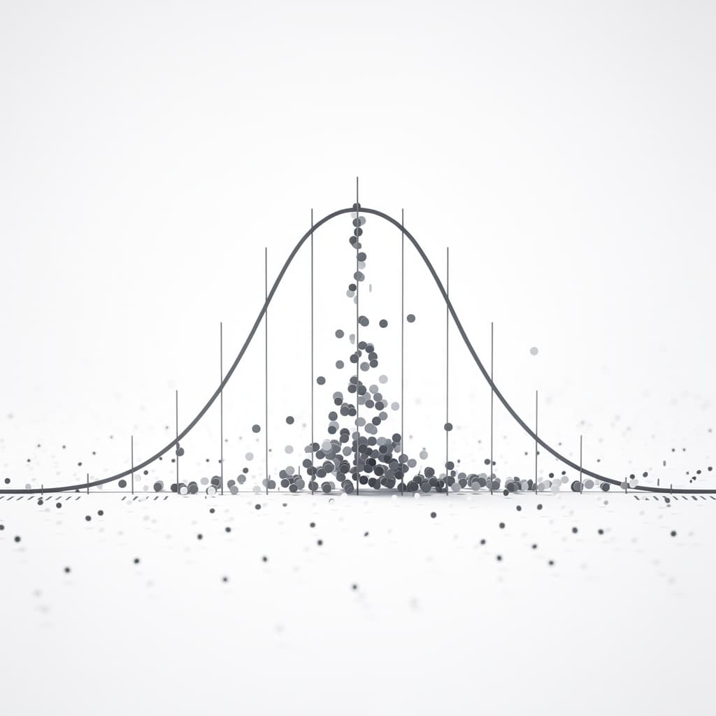
Foundations of the Gaussian Curve

The mathematical heart of the normal distribution is defined by its Probability Density Function (PDF), a formula that describes the relative likelihood of a random variable taking on a specific value. Unlike discrete distributions where one might count individual occurrences, the normal distribution is continuous, meaning it accounts for an infinite number of possible values within a range. The height of the curve at any given point does not represent a direct probability of that single value, as the probability of any exact point in a continuous field is technically zero. Instead, the area under the curve between two points represents the probability that a value will fall within that specific interval. This relationship is captured by the Gaussian function, which incorporates the mathematical constants $\pi$ and $e$ to create its characteristic smooth, tapering shape.

The behavior of this curve is dictated entirely by two fundamental parameters: the mean ($\mu$) and the variance ($\sigma^2$). The mean serves as the location parameter, determining the horizontal position of the peak and representing the arithmetic average of the distribution. Variance, and its square root, the standard deviation ($\sigma$), acts as the scale parameter, dictating how "spread out" or "pinched" the bell shape appears. A small standard deviation results in a tall, narrow spike where data is tightly clustered around the average, while a large standard deviation produces a short, wide curve where values are more dispersed. The PDF formula that unites these elements is expressed as:

$$f(x) = \frac{1}{\sigma\sqrt{2\pi}} e^{-\frac{1}{2}\left(\frac{x-\mu}{\sigma}\right)^2}$$

Conceptually, the origin of the bell curve is rooted in the early 19th-century work of Carl Friedrich Gauss and Abraham de Moivre. While De Moivre first derived the distribution as an approximation for coin-flipping outcomes, Gauss applied it to the study of errors in planetary observations, realizing that measurement deviations naturally formed this specific symmetric pattern. This historical development shifted the perception of "error" from a nuisance to a mathematically predictable phenomenon. Today, the term Gaussian distribution is used interchangeably with normal distribution in honor of Gauss’s contribution to understanding how independent, random fluctuations aggregate into a stable and elegant structure.

Structural Properties of Normal Distribution

One of the most defining characteristics of the normal distribution is its perfect symmetry around the vertical axis passing through the mean. If one were to fold the curve in half at its peak, the two sides would align perfectly, indicating that values above the mean are just as likely to occur as values below it. This symmetry leads to the unique property where the mean, median, and mode are all identical and located at the center of the distribution. In many other types of data distributions, such as those that are "skewed" toward one end, these three measures of central tendency diverge, but in a perfectly normal world, the most frequent value is also the exact middle value and the mathematical average.

The Empirical Rule, also known as the 68-95-99.7 rule, provides a practical framework for visualizing how data is partitioned within this symmetry. According to this rule, approximately 68 percent of all observations in a normal distribution fall within one standard deviation ($\pm 1\sigma$) of the mean. This concentration increases rapidly as the range widens, with 95 percent of data falling within two standard deviations ($\pm 2\sigma$) and 99.7 percent falling within three standard deviations ($\pm 3\sigma$). This rule is a cornerstone of bell curve explained literature, as it allows anyone to quickly estimate the rarity of an observation if they know the mean and standard deviation of the dataset.

Another critical structural feature is the asymptotic behavior of the curve's tails, which extend infinitely in both directions. While the height of the curve drops precipitously as one moves away from the mean, it theoretically never touches the horizontal axis (the x-axis). This implies that while extremely distant outliers—such as a human being ten feet tall—are astronomically improbable, the mathematical model does not strictly rule them out as impossible. This infinite nature ensures that the total area under the entire curve always sums to exactly one, representing the 100 percent probability that a random variable will take on some real value. This structural integrity makes the normal distribution a robust tool for calculating risks and probabilities even in the most extreme edge cases.

The Standard Normal Distribution Framework

While there are an infinite number of possible normal distributions based on different means and deviations, the standard normal distribution serves as a universal benchmark for comparison. Defined as having a mean of zero ($\mu = 0$) and a standard deviation of one ($\sigma = 1$), this specific form is often denoted by the letter $Z$. The standard normal distribution allows statisticians to translate data from completely different scales—such as comparing a student's score on a math test to their score on a chemistry test—into a single, unified metric. By centering the distribution at zero, we create a reference point where positive values represent results above average and negative values represent results below average.

The geometry of the unit curve is particularly useful because the areas under this specific curve have been pre-calculated and recorded in Z-tables. In the era before high-speed computing, these tables were the primary tool for determining probabilities, allowing researchers to find the exact area to the left or right of any given point. Because the total area is one and the curve is symmetric, the area to the left of the mean is always 0.5. If a researcher knows that a specific point on the unit curve is 1.96 standard deviations from the zero-center, they can instantly determine that only 2.5 percent of the distribution lies beyond that point in the upper tail. This geometric consistency is what enables the high degree of precision required in modern scientific research.

Transitioning from a general normal distribution to a standard normal distribution is a process known as standardization. This transformation effectively "re-scales" any normal distribution so that it fits the $N(0, 1)$ mold without changing the relative positioning of the data points. Whether the original data measured temperatures in Celsius, weights in kilograms, or time in seconds, the standardized version strips away the units to focus purely on the probability of the outcome. This abstraction is vital for the z-score formula, which acts as the bridge between raw data and standardized probability, ensuring that statistical logic remains consistent across all fields of study.

Quantifying Deviation with the Z-Score Formula

To understand where a specific data point stands in relation to the rest of the population, we use a calculation known as the z-score formula. This mathematical operation determines exactly how many standard deviations an observation is away from the mean, providing a "relative position" that is much more informative than the raw value alone. For example, knowing that a person's cholesterol level is 220 might be meaningless without context, but knowing they have a Z-score of +2.5 immediately signals that their level is significantly higher than the average. The formula is elegantly simple, requiring only the individual value ($x$), the population mean ($\mu$), and the standard deviation ($\sigma$):

$$z = \frac{x - \mu}{\sigma}$$

The logic of this normalization process is to eliminate the influence of different units and scales. When we subtract the mean from a raw value, we are "centering" the data by seeing how far it deviates from the "norm." When we then divide that difference by the standard deviation, we are "scaling" that deviation into units of standard deviation. If the resulting Z-score is zero, the data point is exactly average; if it is positive, it is above average; and if it is negative, it is below average. Most observations in a normal distribution will result in Z-scores between -3 and +3, reflecting the 99.7 percent probability dictated by the Empirical Rule.

Interpreting these scores often involves using a Z-table or a statistical software package to find the cumulative probability. A cumulative probability tells us the percentage of the population that falls below a certain Z-score. For instance, a Z-score of +1.0 corresponds to a cumulative probability of approximately 0.8413, meaning that roughly 84 percent of the population has a value lower than that specific point. This quantification is the "bread and butter" of standardized testing, quality control in manufacturing, and medical diagnostics, as it provides a clear, objective threshold for what constitutes an "outlier" or a "significant" result in any given context.

The Central Limit Theorem and Emergence

One might wonder why the bell shape is so ubiquitous in the natural world; the answer lies in a powerful mathematical principle known as the Central Limit Theorem (CLT). The CLT states that when you add together a large number of independent, identically distributed random variables, their normalized sum tends toward a normal distribution, regardless of the shape of the original distribution. This means that even if the underlying individual factors are chaotic, skewed, or uniform, their collective average will almost always form a symmetric bell curve as the sample size increases. This convergence is the "magic" of statistics, explaining why complex systems with many small, interacting parts eventually settle into a predictable pattern.

A classic visual demonstration of this emergence is the Galton Board, a vertical board with rows of pegs where balls are dropped from the top. As each ball hits a peg, it has a 50 percent chance of bouncing left or right; though each ball's individual path is random, the thousands of balls eventually accumulate into a perfect bell curve at the bottom. This physical analogy mirrors how human traits like height are determined. Height is not controlled by a single gene, but by the additive effect of hundreds of genetic and environmental factors; because these factors are independent and numerous, the resulting distribution of heights across a population is remarkably normal.

In the world of professional research, the CLT is the reason sampling distributions are so vital. When researchers take multiple samples from a population and calculate the mean of each sample, those sample means will form a normal distribution even if the population they came from is not normal. This allows scientists to use normal distribution examples to make inferences about populations that would otherwise be mathematically difficult to handle. Because we know the "shape" of how sample means behave, we can calculate the probability that our specific sample is a fluke or a genuine representation of the whole, forming the basis for nearly all hypothesis testing.

Normal Distribution Examples in Reality

The properties of normal distribution are not just theoretical abstractions; they are visible in almost every facet of our physical existence. In biology, many human traits like blood pressure, IQ scores, and birth weights follow a normal distribution. While an individual's trait is influenced by a unique combination of genetics and lifestyle, the aggregate of these millions of independent variables results in a population where most people are "average" and fewer people exist at the extremes. For example, the distribution of adult male heights in many countries clusters around 175 centimeters, with very few individuals falling below 150 centimeters or above 200 centimeters.

In the physical sciences, the normal distribution is the standard model for measurement errors. When a scientist measures the distance to a star or the mass of a subatomic particle, multiple trials will yield slightly different results due to environmental noise or equipment limitations. These errors are generally random and unbiased, meaning they are just as likely to be slightly too high as they are to be slightly too low. Consequently, when the scientist plots these measurements, they form a bell curve centered on the "true" value. This allows the researcher to report not just a single number, but a "confidence interval" that describes the precision of their findings.

The world of finance and economics also relies heavily on the normal distribution, though with important caveats. Many financial models, such as the Black-Scholes model for pricing options, assume that the returns on assets follow a normal (or log-normal) distribution. This assumption allows banks and investors to calculate market risk and the probability of large losses. However, critics often point out that financial markets frequently experience "fat tails"—extreme events like market crashes that happen more often than the normal distribution would predict. Despite these limitations, the Gaussian model remains the starting point for risk management because it provides a clear baseline for what "stable" behavior looks like.

Inference and Hypothesis Testing Logic

The ultimate utility of the normal distribution lies in its role in statistical inference, the process of using data from a small sample to make broad claims about a whole population. This is achieved through the construction of confidence intervals, which provide a range of values within which we are reasonably certain the true population parameter lies. For example, a political poll might state that a candidate has 52 percent support with a "margin of error" of plus or minus 3 percent. This margin of error is calculated using the properties of the normal distribution, specifically identifying the Z-score that corresponds to a 95 percent confidence level.

In formal scientific research, the normal distribution is used to determine significance levels and calculate p-values. When a researcher tests a new drug, they start with a "null hypothesis" that the drug has no effect. They then calculate the probability of seeing their experimental results—or something more extreme—given that the null hypothesis is true. If that probability (the p-value) is very low, typically less than 0.05, it means the result falls in the "tails" of the normal distribution. This suggests that the observed effect is unlikely to be the result of random chance alone, leading the researcher to "reject the null hypothesis" and claim a significant discovery.

This logical framework relies on the assumption that the sampling distribution of the test statistic is normal. By identifying "critical regions" in the tails of the bell curve, statisticians can set strict thresholds for proof. If a result falls beyond a certain Z-score (like 1.96 for a two-tailed 95 percent test), it is deemed statistically significant. This rigorous application of the Gaussian curve ensures that science remains objective, preventing researchers from being fooled by random fluctuations and providing a standardized way to communicate the strength of evidence across different disciplines. Through this probabilistic logic, the normal distribution transforms raw, messy data into structured, actionable knowledge.

References

- Stigler, S. M., "The History of Statistics: The Measurement of Uncertainty before 1900", Harvard University Press, 1986.
- Gauss, C. F., "Theoria motus corporum coelestium in sectionibus conicis solem ambientium", Perthes et Besser, 1809.
- Feller, W., "An Introduction to Probability Theory and Its Applications", Wiley, 1968.
- Casella, G., & Berger, R. L., "Statistical Inference", Duxbury Press, 2002.
Recommended Readings
- The Drunkard's Walk: How Randomness Rules Our Lives by Leonard Mlodinow — An engaging exploration of how probability and the normal distribution shape our daily experiences and misconceptions about luck.
- The Lady Tasting Tea by David Salsburg — A historical narrative that explains how the normal distribution and other statistical tools revolutionized science in the 20th century.
- Against the Gods: The Remarkable Story of Risk by Peter L. Bernstein — A comprehensive look at the history of risk management and the mathematical discovery of the bell curve's predictive power.
- Standard Deviations: Flaws and Fallacies in Data Analysis by Gary Smith — A critical look at how the normal distribution is sometimes misapplied in finance and social science, providing essential context for real-world data.