The Elegant Logic of Quadratic Equations

The study of quadratic equations represents a pivotal transition in mathematical education, moving from the linear simplicity of basic arithmetic to the nuanced curves of analytical geometry. These equations, characterized by a single variable raised to the second power, serve as the foundational language for describing physical phenomena ranging from the trajectory of a thrown ball to the optimal pricing strategies in economics. Understanding how to solve quadratic equations is more than a procedural requirement; it is an exercise in logic that bridges the gap between abstract symbolic manipulation and the visual reality of the Cartesian plane. By mastering the various methods of solution, from factoring to the universal quadratic formula, a student gains the tools necessary to decode the behavior of parabolas and the intricate relationships between algebraic coefficients and their geometric counterparts.

Anatomy of the Second-Degree Polynomial

The Standard Algebraic Form

A quadratic equation is formally defined as a second-degree polynomial equation in a single variable, typically written in the standard form $$ax^2 + bx + c = 0$$. In this expression, $x$ represents the unknown value we seek, while $a$, $b$, and $c$ are known numerical constants, with the critical constraint that $a$ cannot equal zero. If $a$ were zero, the $x^2$ term would vanish, reducing the expression to a first-degree linear equation. The term $ax^2$ is known as the quadratic term, $bx$ as the linear term, and $c$ as the constant term, each contributing distinct characteristics to the resulting mathematical model. Historically, the pursuit of solutions for these equations dates back to ancient Babylonian and Egyptian civilizations, though the symbolic notation used today was refined during the Islamic Golden Age and the European Renaissance.

Coefficients and Their Influence

The coefficients $a$, $b$, and $c$ are the genetic markers of the quadratic equation, dictating the shape, position, and orientation of the resulting parabola. The leading coefficient, a, determines the "width" and the direction of the parabola’s opening; a positive $a$ results in a bowl-like shape opening upward, while a negative $a$ creates a mountain-like shape opening downward. The linear coefficient, b, influences the horizontal position of the parabola's vertex, working in tandem with $a$ to shift the axis of symmetry across the coordinate plane. Finally, the constant term, c, represents the $y$-intercept of the function, indicating exactly where the curve crosses the vertical axis when $x$ is zero. This structural understanding is essential because it allows mathematicians to predict the behavior of a system before any rigorous calculation begins, turning raw numbers into an intuitive visual map.

Factoring Quadratic Equations for Simplicity

The Zero Product Property

The most elegant approach to factoring quadratic equations relies on a fundamental principle of arithmetic known as the Zero Product Property. This property states that if the product of two real numbers or algebraic expressions is zero, then at least one of those factors must themselves be zero. When we rewrite a quadratic equation from its standard form into a factored form such as $a(x - r_1)(x - r_2) = 0$, we transform a complex addition problem into a simple logic puzzle. By setting each binomial factor equal to zero—$x - r_1 = 0$ and $x - r_2 = 0$—we can immediately identify the roots of the equation as $r_1$ and $r_2$. This method is highly efficient for equations with integer coefficients that lend themselves to easy decomposition, providing a clear and direct path to the solution without the need for complex radicals.

Binomial Expansion in Reverse

To factor a quadratic where the leading coefficient $a = 1$, we look for two numbers that simultaneously satisfy two conditions: they must multiply to equal the constant $c$ and add together to equal the linear coefficient $b$. This process is essentially the inverse of the FOIL (First, Outer, Inner, Last) method used in binomial expansion. For example, in the equation $x^2 + 5x + 6 = 0$, we seek two numbers that multiply to 6 and add to 5, which are 2 and 3. Thus, the equation is rewritten as $(x + 2)(x + 3) = 0$, leading to the solutions $x = -2$ and $x = -3$. When the leading coefficient $a$ is greater than one, the process becomes slightly more involved, often requiring a technique called factoring by grouping or the "ac method," where we multiply $a$ and $c$ and find factors that sum to $b$ to split the middle term into two parts.

Completing the Square Step by Step

Establishing the Perfect Square

When an equation cannot be easily factored, completing the square step by step offers a robust alternative that relies on the creation of a perfect square trinomial. A perfect square trinomial is an algebraic expression that can be written as the square of a binomial, such as $x^2 + 2dx + d^2 = (x + d)^2$. The goal of this method is to manipulate the standard form $ax^2 + bx + c = 0$ so that the left side of the equation becomes such a square, allowing us to solve for $x$ by taking the square root of both sides. This technique is theoretically significant because it serves as the algebraic proof used to derive the universal quadratic formula. It forces the equation into a structure that isolates the variable, providing a clear view of how the constants relate to the central axis of the parabola.

Algebraic Balancing Techniques

The procedure begins by ensuring the leading coefficient $a$ is equal to 1, which is achieved by dividing the entire equation by $a$ if necessary. Next, the constant term $c$ is moved to the right side of the equation, leaving $x^2 + (b/a)x$ on the left. To "complete the square," we take half of the coefficient of $x$, square it, and add that value to both sides of the equation to maintain balance. For an equation $x^2 + 6x = 7$, we take half of 6 (which is 3), square it (which is 9), and add it to both sides to get $x^2 + 6x + 9 = 16$. This simplifies to $(x + 3)^2 = 16$, and by taking the square root, we find $x + 3 = \pm 4$, resulting in the solutions $x = 1$ and $x = -7$. This method is particularly useful in higher-level mathematics, such as calculus and conic sections, where converting equations into vertex form is necessary for graphing and optimization.

Essential Quadratic Formula Examples

Managing the Radicand

The quadratic formula is the most powerful tool in the mathematician's arsenal for solving second-degree equations, as it provides a solution for any quadratic, regardless of whether the roots are rational, irrational, or complex. The formula is expressed as:

$$x = \frac{-b \pm \sqrt{b^2 - 4ac}}{2a}$$

One of the most critical aspects of applying this formula correctly is the careful management of the radicand—the expression inside the square root symbol ($b^2 - 4ac$). When working through quadratic formula examples, students must be vigilant with the signs of the coefficients, especially when $a$ or $c$ are negative, as a double negative will result in an addition within the square root. Failure to correctly calculate the radicand is the most common source of error in manual computations. By isolating the radicand first, one can determine if the equation will yield real numbers or if it will require the use of imaginary units ($i$) to express the solution.

Solving for Real Intercepts

To illustrate the formula's utility, consider the equation $2x^2 - 5x + 3 = 0$. Here, we identify $a = 2$, $b = -5$, and $c = 3$. Substituting these values into the formula, we begin with the radicand: $(-5)^2 - 4(2)(3)$, which simplifies to $25 - 24 = 1$. Since the square root of 1 is 1, the formula becomes $x = (5 \pm 1) / 4$. This yields two distinct rational solutions: $x = (5 + 1) / 4 = 1.5$ and $x = (5 - 1) / 4 = 1$. This example demonstrates how the formula handles equations that could have been factored, but it does so with a standardized process that requires no "guess and check" logic. In cases where the radicand is not a perfect square, such as 7 or 13, the formula allows us to provide exact answers in radical form, which are far more precise than decimal approximations for scientific calculations.

Decoding the Discriminant Formula

Determining the Nature of Roots

The expression found under the radical in the quadratic formula, $D = b^2 - 4ac$, is known as the discriminant formula. It serves as a diagnostic tool that reveals the nature of the roots without requiring the full solution of the equation. By evaluating the discriminant, we can classify the solutions into three distinct categories based on its value relative to zero. If $D > 0$, the equation possesses two distinct real roots, meaning the parabola crosses the $x$-axis at two different points. If $D = 0$, there is exactly one real root, often called a repeated or double root, which indicates that the vertex of the parabola sits exactly on the $x$-axis. Finally, if $D < 0$, the equation has no real roots, and the solutions are a pair of complex conjugates, signifying that the parabola never touches or crosses the $x$-axis.

Identifying the Vertex Point

Beyond merely counting the roots, the components of the discriminant and the quadratic formula also help us locate the vertex, the highest or lowest point on the parabola. The $x$-coordinate of the vertex is always given by the first part of the quadratic formula: $x = -b / (2a)$. This value represents the axis of symmetry, a vertical line that divides the parabola into two mirrored halves. Once this $x$-coordinate is found, it can be substituted back into the original equation $ax^2 + bx + c$ to find the corresponding $y$-coordinate. Understanding the relationship between the discriminant and the vertex allows for a deeper comprehension of the "gap" between the curve and the $x$-axis; specifically, the discriminant's magnitude tells us how far the vertex is from the axis relative to the steepness of the curve.

Modern Quadratic Equation Calculator Method

Computational Accuracy and Inputs

In contemporary scientific and engineering contexts, the quadratic equation calculator method has become the standard for rapid problem-solving. Whether using a handheld graphing calculator, a specialized software package like MATLAB, or an online computational engine, the process involves inputting the coefficients $a$, $b$, and $c$ into a pre-programmed algorithm. These digital tools eliminate the risk of arithmetic errors and can provide solutions in multiple formats, including exact radicals, decimal approximations, and complex numbers. However, the accuracy of the output is entirely dependent on the "garbage in, garbage out" principle; a single sign error during data entry will result in an entirely incorrect solution. Users must also be aware of the "precision limits" of digital calculators, which may round very small values to zero, potentially obscuring the presence of two very close roots.

Interpreting Digital Solutions

Modern software does more than just provide a numerical answer; it often provides a visual and symbolic context for the solution. For instance, many calculators will automatically graph the function, allowing the user to verify the roots by observing the $x$-intercepts. When a calculator returns a result containing the letter $i$ (e.g., $2 \pm 3i$), it is informing the user that the solution exists in the complex plane, which is vital for fields like electrical engineering and fluid dynamics. Below is a conceptual representation of how a simple computer program might execute the quadratic formula logic:

import math

def solve_quadratic(a, b, c):
    discriminant = b*2 - 4a*c
    
    if discriminant > 0:
        root1 = (-b + math.sqrt(discriminant)) / (2*a)
        root2 = (-b - math.sqrt(discriminant)) / (2*a)
        return root1, root2
    elif discriminant == 0:
        return -b / (2*a)
    else:
        real_part = -b / (2*a)
        imag_part = math.sqrt(abs(discriminant)) / (2*a)
        return (f"{real_part} + {imag_part}i", f"{real_part} - {imag_part}i")

Geometric Interpretations of Roots

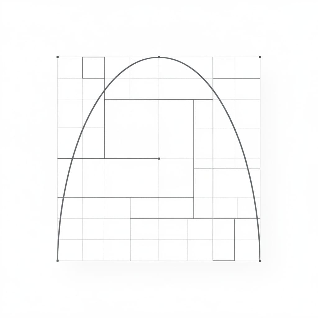
The Parabola on the Cartesian Plane

The most profound way to understand how to solve quadratic equations is to view the roots as geometric intersections. In a two-dimensional Cartesian coordinate system, the quadratic equation $y = ax^2 + bx + c$ describes a parabola. When we set $y = 0$ to solve the equation, we are effectively looking for the points where the parabola intersects the $x$-axis. These points, known as the $x$-intercepts, are the physical manifestation of the algebraic roots. If you imagine the parabola as the path of a projectile, the roots represent the locations where the object is at ground level. The symmetry of the parabola ensures that these roots are always equidistant from the axis of symmetry ($x = -b/2a$), providing a beautiful balance between the left and right sides of the mathematical expression.

Tangency and Intersection Points

The behavior of the parabola relative to the $x$-axis illustrates the logic of the discriminant in a purely visual way. A parabola that is "tangent" to the $x$-axis touches it at exactly one point—the vertex—which corresponds to a discriminant of zero. If the vertex lies below the axis and the parabola opens upward (or vice versa), the curve must cross the axis twice, creating two real roots. Conversely, if the vertex is above the axis and opens upward, the curve "escapes" into the upper quadrants without ever touching the $x$-axis, leading to the complex solutions we observe algebraically. This geometric perspective is crucial for solving real-world optimization problems, such as finding the maximum area that can be enclosed by a certain length of fencing, where the vertex of the quadratic represents the optimal solution.