The Elegant Dynamics of Bernoulli's Equation

The study of fluid dynamics represents one of the most significant chapters in the history of classical physics, bridging the gap between theoretical mechanics and practical engineering. At the heart of this discipline lies Bernoulli's equation, a mathematical statement that describes the conservation of energy within a flowing fluid. Formulated in the 18th century by the Swiss mathematician Daniel Bernoulli, this principle serves as the foundational bedrock for understanding how pressure, velocity, and elevation interact. From the soaring flight of modern aircraft to the intricate plumbing systems within a skyscraper, the dynamics of this equation govern the movement of liquids and gases in our physical world. By treating fluids as a continuous medium where energy is neither created nor destroyed, but merely transformed, engineers can predict the behavior of complex systems with remarkable precision.

Foundations of Fluid Dynamics

Fluid Mechanics Basics and Ideal Systems

To understand the utility of Bernoulli's equation, one must first establish the parameters of the fluid environments where it is most applicable. In the realm of fluid mechanics, an "ideal fluid" is a conceptual model used to simplify the complex realities of molecular interaction. This idealized system assumes that the fluid is incompressible, meaning its density remains constant regardless of the pressure applied, and inviscid, implying that internal friction or "stickiness" is negligible. Furthermore, the flow is assumed to be steady-state, where the velocity and pressure at any fixed point in the system do not change over time. While no real-world fluid is perfectly ideal, water and many gases at low speeds behave sufficiently like ideal fluids to make Bernoulli's insights incredibly accurate for practical engineering applications.

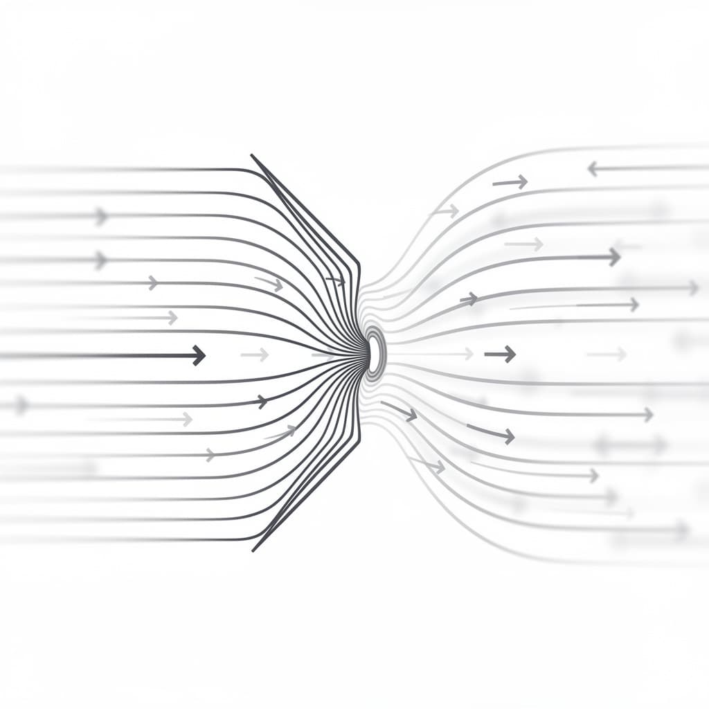
The motion of these fluids is typically visualized through streamlines, which are imaginary lines representing the path of fluid particles in a steady flow. When we analyze a system using Bernoulli's equation, we are essentially tracking the energy of a fluid parcel as it travels along one of these streamlines. Because the flow is steady and non-viscous, there is no loss of energy to heat through friction, and no energy is added by external pumps within the segment being studied. This allows for a closed-loop analysis where the total mechanical energy remains constant. This conceptual framework provides the necessary "laboratory conditions" for the mathematical derivation of flow laws that define everything from the spray of a garden hose to the cooling systems of nuclear reactors.

Energy Conservation in Moving Liquids

The core philosophy of Bernoulli's equation is rooted in the Law of Conservation of Energy, specifically adapted for the unique characteristics of fluids. In a moving fluid, energy exists in three primary forms: kinetic energy due to the fluid's motion, potential energy due to its elevation, and "flow energy" associated with its pressure. As a fluid particle moves through a pipe of varying diameter or height, it may speed up or slow down, and it may rise or fall. According to the conservation principle, if the kinetic energy increases because the fluid speeds up, this energy must be "stolen" from either the potential energy or the pressure of the fluid. This inverse relationship explains why a fluid’s pressure drops when its velocity increases, a phenomenon that often defies the common intuition that "faster means more force."

Consider the analogy of a roller coaster car moving along a track; as it descends a hill, it trades its potential energy for kinetic energy, speeding up as it loses height. In a fluid system, Bernoulli's equation acts as the ledger for this energy trade, but it adds the third variable of pressure. When a fluid enters a narrower section of a pipe (a venturi), it must speed up to maintain the same mass flow rate, a requirement known as the Continuity Equation. Because the fluid's kinetic energy has increased at the constriction, and assuming the height remains the same, the static pressure must drop to balance the energy equation. This interplay between motion and pressure is the fundamental mechanism behind thousands of industrial and natural processes.

The Structure of the Bernoulli Formula

Defining Static and Dynamic Pressure

The mathematical representation of Bernoulli's equation is typically expressed as the sum of three distinct pressure terms that remain constant along a streamline. The standard form of the equation is written as follows:

$$P + \frac{1}{2}\rho v^2 + \rho gh = \text{constant}$$

In this expression, $P$ represents the static pressure, which is the actual thermodynamic pressure of the fluid as it moves. This is the pressure one would measure if moving along with the fluid at the same velocity, or the pressure exerted against the walls of a pipe. Static pressure is a measure of the internal energy of the fluid particles and is the primary driver of flow from high-pressure zones to low-pressure zones.

The second term, $\frac{1}{2}\rho v^2$, is known as the dynamic pressure. This term represents the kinetic energy of the fluid per unit volume, where $\rho$ (rho) is the fluid density and $v$ is the flow velocity. Dynamic pressure is not a "pressure" in the sense of a force pushing against a surface at rest, but rather the potential for pressure that would be realized if the fluid were forced to come to a complete stop. The final term, $\rho gh$, is the hydrostatic pressure, representing the potential energy per unit volume due to the fluid's weight and its height ($h$) above a reference datum. Together, these three terms account for the total mechanical energy density of the fluid at any given point.

Total Pressure and Stagnation Points

The sum of static and dynamic pressure is often referred to as the total pressure or stagnation pressure, specifically in scenarios where the height changes are negligible. Stagnation pressure ($P_0$) is the pressure a fluid reaches when it is brought to rest isentropically (without any loss). This concept is vital in aerodynamics, particularly at the nose of an aircraft or the leading edge of a wing. At these "stagnation points," the velocity of the air relative to the surface is zero, meaning all the kinetic energy of the oncoming flow has been converted into pressure. Consequently, the stagnation pressure is the highest pressure found anywhere in the flow field surrounding an object.

Understanding the distinction between these pressures is crucial for instrumentation and system design. For example, if an engineer needs to measure the speed of a liquid in a pipe, they cannot simply use a standard pressure gauge, as that only measures static pressure. Instead, they must use a device that can compare the static pressure to the total pressure. The difference between the two is the dynamic pressure, which can then be used to solve for the velocity $v$. This relationship highlights the elegance of Bernoulli's equation: it turns a difficult-to-measure variable (velocity) into a more manageable measurement of pressure differences.

A Systematic Derivation of the Equation

The Work-Energy Theorem for Streamlines

The most common way to derive Bernoulli's equation is through the Work-Energy Theorem, which states that the work done on a system by external forces is equal to the change in the system's kinetic and potential energy. Imagine a small "plug" or segment of fluid moving through a pipe with a varying cross-sectional area. As the fluid moves from position 1 to position 2, the fluid behind it exerts a force ($F_1 = P_1 A_1$) doing positive work, while the fluid ahead of it exerts a resistive force ($F_2 = P_2 A_2$) doing negative work. The net work done by these pressure forces over a small distance $\Delta x$ is $(P_1 A_1 \Delta x_1 - P_2 A_2 \Delta x_2)$. Since $A \Delta x$ represents the volume of the fluid segment ($\Delta V$), the work can be simplified to $(P_1 - P_2) \Delta V$.

Next, we account for the changes in mechanical energy. The change in kinetic energy is $\frac{1}{2} m (v_2^2 - v_1^2)$, and the change in gravitational potential energy is $mg(h_2 - h_1)$. By substituting mass ($m$) with density times volume ($\rho \Delta V$), we can equate the net work to the sum of these energy changes. When we divide the entire equation by the volume $\Delta V$, the volume term cancels out, leaving us with a relationship defined purely by pressure, density, velocity, and height. Rearranging the terms so that all variables associated with position 1 are on one side and position 2 on the other yields the familiar constant-sum form of the equation. This derivation reinforces the idea that pressure is effectively "potential energy per unit volume."

Mathematical Integration of Euler Equations

For a more rigorous fluid-mechanical perspective, Bernoulli's equation can be derived by integrating the Euler equations of motion. The Euler equations are a set of partial differential equations that describe the motion of an inviscid, incompressible fluid based on Newton's Second Law ($F = ma$). For steady flow along a streamline, the acceleration of a fluid particle can be expressed in terms of the gradient of its velocity. When we analyze the forces acting along a streamline—specifically the pressure gradient and the component of gravity—we arrive at a differential equation relating $dP$, $v dv$, and $dh$.

By integrating this differential equation along the path of the flow, the constant of integration appears as the "Bernoulli constant." The integration process assumes that the density is constant (incompressible flow) and that the only work-producing forces are pressure and gravity. This approach is powerful because it demonstrates that the equation is not just a high-level energy balance, but a direct consequence of local force balances acting on every individual fluid particle. It also clarifies why the equation is technically only valid "along a streamline," as the constant may differ between different streamlines in a flow field that has rotation or "vorticity."

Bernoulli's Equation Units and Dimensions

Standard SI and Imperial Units

To use Bernoulli's equation effectively in engineering, one must be meticulous with units to ensure that every term in the sum is compatible. In the International System of Units (SI), the most common units are as follows:

Variable	Description	SI Unit	Imperial Unit
$P$	Static Pressure	Pascals ($Pa$ or $N/m^2$)	Pounds per sq. foot ($lb/ft^2$ or $psf$)
$\rho$	Fluid Density	Kilograms per cubic meter ($kg/m^3$)	Slugs per cubic foot ($slugs/ft^3$)
$v$	Flow Velocity	Meters per second ($m/s$)	Feet per second ($ft/s$)
$g$	Gravity	$9.81 m/s^2$	$32.2 ft/s^2$
$h$	Elevation	Meters ($m$)	Feet ($ft$)

When calculating the dynamic pressure term ($\frac{1}{2}\rho v^2$) in SI, the result will be in $(kg/m^3) \cdot (m/s)^2$. Breaking down the units, this simplifies to $kg \cdot m / (s^2 \cdot m^2)$, which is $N/m^2$, or Pascals. It is a common mistake in the United States to use "pounds per square inch" (psi) for pressure while using "feet" for elevation. To avoid errors, all pressure terms must be converted to a consistent base—typically $psf$ in the Imperial system—before the final calculation is performed.

Ensuring Dimensional Homogeneity

Dimensional homogeneity is the principle that every term in a physical equation must have the same dimensions. In Bernoulli's equation, every term has the dimensions of pressure, which is defined as force per unit area $[M L^{-1} T^{-2}]$. Alternatively, if we divide the entire equation by the specific weight of the fluid ($\gamma = \rho g$), we get what civil engineers refer to as the "Head" form of the equation. This version is particularly popular in hydraulics and water management because every term is expressed in units of length (meters or feet).

The "Head" form of the equation is written as:

$$\frac{P}{\rho g} + \frac{v^2}{2g} + h = H$$

Here, $\frac{P}{\rho g}$ is the pressure head, representing the height of a column of fluid that would exert that amount of pressure. The term $\frac{v^2}{2g}$ is the velocity head, and $h$ is the elevation head. The sum $H$ is the total head. Using dimensions of length makes it much easier for engineers to visualize energy levels in a reservoir or piping system, as the total head represents the maximum height the fluid could reach if all its energy were converted back into potential energy. This version of the equation is the standard for designing pumps and determining the "hydraulic grade line" of municipal water systems.

Aviation and Aerodynamic Applications

Generating Lift Through Pressure Differentials

Perhaps the most famous application of Bernoulli's equation is the explanation of how airplane wings generate lift. While lift is a complex phenomenon involving both Bernoulli's principle and Newton's Third Law (downwash), the pressure differential described by Bernoulli is a major component. An airfoil (the shape of a wing) is designed so that the air traveling over the curved top surface must travel faster than the air moving across the relatively flat bottom. According to the equation, since the air on top is moving at a higher velocity, its static pressure must be lower than the pressure of the slower-moving air underneath. This pressure imbalance creates a net upward force known as lift.

This principle is not limited to aircraft; it also explains the behavior of a spinning ball in sports, known as the Magnus effect. When a soccer ball or baseball spins, it drags a layer of air around with it. On one side of the ball, the spin is moving in the same direction as the oncoming air, increasing the local air velocity. On the opposite side, the spin opposes the air, decreasing the velocity. The resulting pressure difference—lower pressure on the high-velocity side—causes the ball to curve in flight. Whether in the design of a Boeing 747 wing or a professional pitcher's curveball, the manipulation of velocity to control pressure is a fundamental tactic in aerodynamics.

The Function of Pitot-Static Systems

Pilots rely on Bernoulli's equation every time they look at their airspeed indicator. This instrument is connected to a Pitot-static system, which consists of a Pitot tube facing directly into the oncoming airflow and static ports located on the side of the fuselage. The Pitot tube captures the stagnation pressure (total pressure), while the static ports measure the ambient atmospheric pressure (static pressure). The airspeed indicator is essentially a differential pressure gauge that subtracts the static pressure from the total pressure to find the dynamic pressure.

Once the dynamic pressure is known, the equation can be rearranged to solve for velocity: $v = \sqrt{2(P_{total} - P_{static}) / \rho}$. This calculation gives the "indicated airspeed" of the aircraft. It is important to note that as a plane climbs higher, the air density ($\rho$) decreases, which is why pilots must differentiate between indicated airspeed and "true airspeed." Without the reliable application of Bernoulli's principles through these physical sensors, safe flight would be impossible, as pilots would have no precise way of knowing if they were flying fast enough to maintain lift or approaching a dangerous stall.

Industrial Bernoulli's Equation Examples

Venturi Meters and Flow Measurement

In industrial processing, accurately measuring the flow rate of chemicals, oils, or gases in a closed pipe is essential for safety and quality control. One of the most reliable devices for this is the Venturi meter, which consists of a converging section, a narrow throat, and a diverging section. As the fluid passes through the narrow throat, its velocity increases due to the continuity of mass. By measuring the pressure at the wide inlet and the narrow throat, engineers can use Bernoulli's equation to calculate the flow velocity without ever needing to place a moving mechanical sensor inside the fluid stream.

The beauty of the Venturi meter lies in its lack of moving parts and its relative efficiency. While there is always some energy lost to friction (which engineers account for using a "discharge coefficient"), the pressure drop in the throat is almost entirely recovered as the pipe widens again. This is a direct real-world demonstration of the "Bernoulli effect." Similar devices, like orifice plates and flow nozzles, work on the same principle: creating a known velocity change and measuring the resulting pressure change to deduce the volume of fluid moving through the system per second.

The Physics of Siphoning and Drainage

The common siphon is another practical example that relies on the relationship between pressure, height, and atmospheric force. To start a siphon, one must fill a tube with liquid and place one end in a higher reservoir and the other in a lower one. The weight of the liquid in the longer, lower arm of the tube creates a region of low pressure at the crest of the siphon. Atmospheric pressure pushing down on the surface of the upper reservoir then forces the liquid up into the tube to fill this low-pressure zone. Bernoulli's equation allows us to calculate the velocity of the discharge at the bottom end, a result known as Torricelli’s Law: $v = \sqrt{2gh}$, where $h$ is the vertical distance from the liquid surface to the outlet.

This same logic applies to the drainage of large tanks and reservoirs. If a hole is poked in the side of a water tank, the speed at which the water exits depends solely on the height of the water above the hole. It does not matter how wide the tank is; a 10-meter deep swimming pool and a 10-meter deep thin pipe will both eject water from a bottom valve at the same speed. This realization is vital for hydraulic engineers designing dam spillways or municipal drainage systems, as it defines the maximum possible flow rate a system can handle under gravity alone.

Assumptions and Physical Limitations

Incompressible and Inviscid Flow Criteria

While Bernoulli's equation is exceptionally versatile, it is not a universal law of nature. It is an approximation that holds true only under specific conditions. The first major assumption is that the fluid is incompressible. For liquids like water or oil, this is generally a safe assumption. However, for gases like air, density can change significantly if the flow reaches high speeds (typically above Mach 0.3). When air is compressed, it stores energy through temperature and density changes, which Bernoulli's basic equation does not account for. In these cases, engineers must use the "compressible Bernoulli equation" or more advanced gas dynamics equations.

The second major limitation is the inviscid assumption, which assumes the fluid has no viscosity. In reality, all fluids have some internal friction. As a fluid flows through a long pipe, it loses energy to the walls in the form of heat, leading to a "pressure drop" that Bernoulli's equation would not predict. For "thick" or highly viscous fluids like honey or heavy crude oil, the equation becomes highly inaccurate. To bridge this gap, engineers use the "Extended Bernoulli Equation," which adds terms for "head loss" due to friction and "pump head" for energy added to the system by mechanical means.

Steady-State vs Unsteady-State Analysis

Finally, the standard form of Bernoulli's equation assumes steady flow. This means the flow pattern does not change over time. If you suddenly open or close a valve, or if a pump is oscillating, the flow is in an "unsteady" state. During these transitions, the fluid experiences local accelerations that require extra force. This leads to phenomena like "water hammer," a pressure surge that occurs when a fluid in motion is forced to stop or change direction suddenly. While there are unsteady versions of the equation that include a time-derivative term ($\int \frac{\partial v}{\partial t} ds$), they are significantly more complex and move into the territory of the full Navier-Stokes equations.

Despite these limitations, Bernoulli's equation remains the first tool an engineer reaches for when analyzing a fluid system. Its power lies in its simplicity and the deep physical intuition it provides. By understanding that pressure, velocity, and height are simply different currencies in a single energy economy, we gain the ability to master the behavior of the fluids that power our machines and sustain our lives. Whether we are measuring the flow of blood through an artery or the flow of air over a supersonic wing, Bernoulli's insights provide the framework upon which all modern fluid dynamics is built.

References

- White, F. M., Fluid Mechanics, McGraw-Hill Education, 2015.
- Munson, B. R., Young, D. F., & Okiishi, T. H., Fundamentals of Fluid Mechanics, Wiley, 2012.
- Bernoulli, D., "Hydrodynamica, sive de viribus et motibus fluidorum commentarii", Johannis Reinholdi Dulseckeri, 1738.
- Anderson, J. D., Fundamentals of Aerodynamics, McGraw-Hill Education, 2016.
- Çengel, Y. A., & Cimbala, J. M., Fluid Mechanics: Fundamentals and Applications, McGraw-Hill, 2017.
Recommended Readings
- The Simple Science of Flight by Henk Tennekes — A fascinating exploration of aerodynamics that explains the principles of lift and Bernoulli's equation using examples from both nature and engineering.
- Flow by Philip Ball — A deep dive into the patterns of nature and the physics of fluids, offering a more conceptual and visual understanding of how liquids and gases move.
- Fluid Mechanics by Pijush K. Kundu and Ira M. Cohen — An advanced textbook that provides the rigorous mathematical derivations for Euler and Navier-Stokes equations for those seeking a deeper dive into the calculus of flow.