Standard Deviation: Definition, Formula, and Step-by-Step Calculation Guide

The concept of standard deviation serves as the cornerstone of modern statistical analysis, providing a precise mathematical measure of how much a set of data fluctuates around its average value. While the arithmetic mean offers a snapshot of the central tendency of a group, it fails to describe whether the individual data points are tightly clustered or widely scattered. Standard deviation bridges this gap by quantifying the degree of dispersion, allowing researchers to determine the reliability and consistency of their observations. In essence, it transforms a collection of raw numbers into a narrative about stability, risk, and predictability within any given system.

Defining Standard Deviation and Statistical Variance

To understand standard deviation, one must first grasp the broader concept of statistical dispersion, which describes the extent to which a distribution is stretched or squeezed. In any dataset, the individual values rarely align perfectly with the mean; instead, they exhibit variability due to inherent randomness or underlying environmental factors. Standard deviation provides a standardized metric to express this variability in the same units as the original data. This makes it far more intuitive than other measures of spread, such as range, which only considers the extreme values and ignores the behavior of the data in between.

The relationship between the mean and variability is fundamental to interpreting the "health" of a dataset. If a group of students takes a test and the average score is 80, a low standard deviation suggests that most students scored very close to 80, indicating a consistent level of understanding across the class. Conversely, a high standard deviation would reveal a significant gap between high-performing and struggling students, even if the average remains exactly the same. Therefore, the mean tells us where the center is, but the standard deviation tells us how much we can actually trust that center to represent any single individual in the group.

Interpreting the result of a standard deviation calculation requires a contextual understanding of the subject matter. A standard deviation of five might be considered negligible when measuring the heights of skyscrapers in meters, but it would be massive if applied to the precision of a microscopic surgical instrument. It is generally understood that a smaller standard deviation indicates higher precision and less "noise" in the data, whereas a larger value suggests a more diverse or volatile environment. By examining the standard deviation, statisticians can identify outliers—data points that fall significantly far from the mean—which often warrant further investigation to determine if they are errors or significant discoveries.

The Standard Deviation Formula Explained

The mathematical representation of standard deviation differs slightly depending on whether one is analyzing an entire population or just a representative sample. For a population standard deviation, we use the Greek letter sigma ($\sigma$) to denote the value. This formula assumes that every possible member of the group has been measured, leaving no room for sampling error. The equation is expressed as:

$$\sigma = \sqrt{\frac{\sum_{i=1}^{N} (x_i - \mu)^2}{N}}$$

In this equation, $x_i$ represents each individual value, $\mu$ is the population mean, and $N$ is the total number of observations. The numerator, known as the sum of squares, captures the total squared distance of all points from the center, which is then averaged and square-rooted to return to the original scale.

When dealing with a subset of a larger group, we use the sample standard deviation formula, denoted by the letter $s$. The primary difference in this equation is the use of $n-1$ in the denominator instead of $N$, a modification known as Bessel's Correction. The formula is written as:

$$s = \sqrt{\frac{\sum_{i=1}^{n} (x_i - \bar{x})^2}{n-1}}$$

Here, $\bar{x}$ represents the sample mean and $n$ is the sample size. This adjustment is necessary because samples tend to naturally underestimate the variability of the full population, and dividing by a slightly smaller number ($n-1$) compensates for this bias, providing a more accurate estimate of the population's true dispersion.

The mathematical constants and operators within these equations serve specific logical purposes that ensure the final result is meaningful. The summation symbol ($\sum$) instructs the mathematician to aggregate the differences for every data point, ensuring no value is excluded from the measure of spread. The squaring of the term $(x_i - \mu)$ is critical because it eliminates negative values; without squaring, the positive and negative deviations would cancel each other out, resulting in a sum of zero. Finally, the square root operation at the end is essential for "undoing" the squaring process, allowing the final result to be expressed in the same units—such as dollars, centimeters, or seconds—as the original dataset.

How to Calculate Standard Deviation Manually

Computing the standard deviation by hand is a rigorous process that begins with finding the arithmetic mean. To calculate the mean, one must sum all the individual observations in the dataset and divide that total by the number of observations ($n$ or $N$). This value serves as the "anchor" for the rest of the calculation, representing the point from which all deviations will be measured. For example, in a small dataset of $\{4, 8, 6, 10\}$, the sum is 28, and the mean is 7. Accurate mean calculation is vital, as any error at this initial stage will propagate through every subsequent step of the formula.

Once the mean is established, the next phase involves calculating the deviation for each data point and squaring those scores. Subtract the mean from each individual value to find the "deviation score," which may be positive or negative depending on whether the value is above or below the average. Squaring these scores is the step that grants standard deviation its mathematical power, as it treats a deviation of -2 and +2 as equally significant. Following the previous example, the deviations from the mean of 7 are $\{-3, 1, -1, 3\}$, and their squares are $\{9, 1, 1, 9\}$. This process emphasizes larger deviations, meaning a single extreme outlier will have a disproportionately large impact on the final standard deviation.

The final stage of manual calculation involves averaging these squared deviations and applying root extraction techniques. If we are treating our example as a population, we sum the squared deviations ($9+1+1+9 = 20$) and divide by the count ($N=4$), resulting in a variance of 5. To convert this back into a usable metric, we take the square root of 5, which is approximately 2.23. If we were treating it as a sample, we would divide by $n-1$ (which is 3), giving a variance of 6.67 and a sample standard deviation of approximately 2.58. This final extraction is what transforms the abstract "squared units" back into a concrete measure of spread that matches the original data's scale.

Essential Standard Deviation Steps for Data Analysis

For professionals working with larger datasets, constructing a deviation table is the most effective way to organize the calculation and prevent algebraic errors. A standard table consists of three columns: the raw data ($x$), the deviation from the mean ($x - \mu$), and the squared deviation $(x - \mu)^2$. By listing every observation in the first column, an analyst can methodically fill out the subsequent columns row by row. This structured approach is particularly helpful when double-checking work, as the sum of the second column (the raw deviations) should always equal zero. If it does not, the analyst knows immediately that the mean was calculated incorrectly or a subtraction error occurred.

Calculating the variance component is the penultimate step in the data analysis workflow. Variance is defined as the average of the squared differences from the mean, and while it is useful in certain statistical proofs, it is often difficult to interpret on its own because its units are squared. For instance, if you are measuring the weight of apples in grams, the variance would be expressed in "square grams," a unit that has no physical meaning in the real world. Despite this, the variance is a critical intermediate value that describes the total power of the fluctuations within the system before the final square root is applied. It serves as a bridge between the raw sum of squares and the final standard deviation.

Summing the squared differences is the core operation that defines the magnitude of the standard deviation. This sum, often abbreviated as $SS$ for "Sum of Squares," represents the total amount of variation present in the dataset. A small $SS$ indicates that the data points are huddled closely around the average, suggesting a high degree of uniformity. A large $SS$ reveals that the data is spread out, indicating either a diverse range of outcomes or a high level of uncertainty in the measurements. By focusing on the sum of squares, analysts can compare the total variability of two different datasets even before they finalize the standard deviation calculation.

Population vs Sample Standard Deviation Differences

The decision to use the population or sample standard deviation depends entirely on the scope of the research and the availability of data. One should use the population standard deviation when the dataset includes every single member of the group being studied. For example, if a teacher wants to find the standard deviation of grades for a specific class of 20 students, that class is the entire population of interest. In this scenario, there is no need to estimate or infer; the data is complete, and dividing by $N$ provides the exact measure of dispersion for that specific group. Population statistics are most common in localized settings, census data, or controlled laboratory environments where every variable is accounted for.

Practical uses for sample statistics arise when it is impossible, expensive, or impractical to measure an entire population. If a biologist wants to know the average wingspan of a specific species of bird across an entire continent, they cannot realistically catch and measure every single bird. Instead, they collect a representative sample of perhaps 200 birds and use the sample standard deviation ($s$) to estimate the variability of the millions of birds they didn't measure. In these cases, the sample acts as a proxy for the truth, and the formulaic adjustment (using $n-1$) is a mathematical safeguard against the limitations of partial data. Sample standard deviation is the standard in social sciences, medical trials, and market research.

The necessity of correcting for bias in small samples cannot be overstated, especially when the sample size is under 30. Mathematically, when we take a sample, we are more likely to pick values that are near the center of the population and less likely to pick the rare extreme values. Consequently, the range and variance of a sample are almost always smaller than the range and variance of the full population. By using $n-1$ in the denominator, statisticians "inflate" the result slightly to account for this missing variability. As the sample size $n$ grows larger, the difference between dividing by $n$ and $n-1$ becomes negligible, reflecting the fact that larger samples are naturally more representative of the population.

Practical Standard Deviation Examples in Science

In the world of laboratory science, standard deviation is the primary tool used for monitoring the precision of experimental results. When a chemist runs multiple trials of a titration to determine the concentration of a solution, they expect the results to be nearly identical. A low standard deviation across these trials indicates high repeatability, suggesting that the equipment is calibrated and the technique is sound. If the standard deviation is high, it signals a problem with the experimental setup, such as temperature fluctuations or contaminated reagents, prompting the scientist to troubleshoot the process before publishing the findings. Without this metric, "accuracy" would be a matter of guesswork rather than rigorous proof.

Financial asset risk assessment relies heavily on standard deviation to define the concept of volatility. In the context of the stock market, the standard deviation of a stock's annual returns provides a clear picture of the risk associated with that investment. A stock with an average return of 8% and a standard deviation of 2% is considered a "safe" or stable investment, as its returns are unlikely to swing wildly. On the other hand, a stock with the same 8% average return but a standard deviation of 20% is highly volatile, meaning the investor could see massive gains or devastating losses in any given year. Portfolio managers use these calculations to balance high-risk and low-risk assets, ensuring that the overall standard deviation of a client's wealth stays within an acceptable range.

Quality control in engineering utilizes standard deviation to ensure that manufactured parts meet strict safety and functional requirements. In a factory producing steel bolts, every bolt must be almost exactly the same diameter to fit into its designated nut; even a millimeter of deviation could lead to structural failure in a bridge or aircraft. Engineers use Statistical Process Control (SPC) to monitor the standard deviation of the production line in real-time. If the standard deviation begins to trend upward, it indicates that the machinery may be wearing down or the raw materials are inconsistent. By maintaining a standard deviation within a specific "tolerance limit," manufacturers can guarantee the reliability of their products at a massive scale.

Standard Deviation and the Normal Distribution Curve

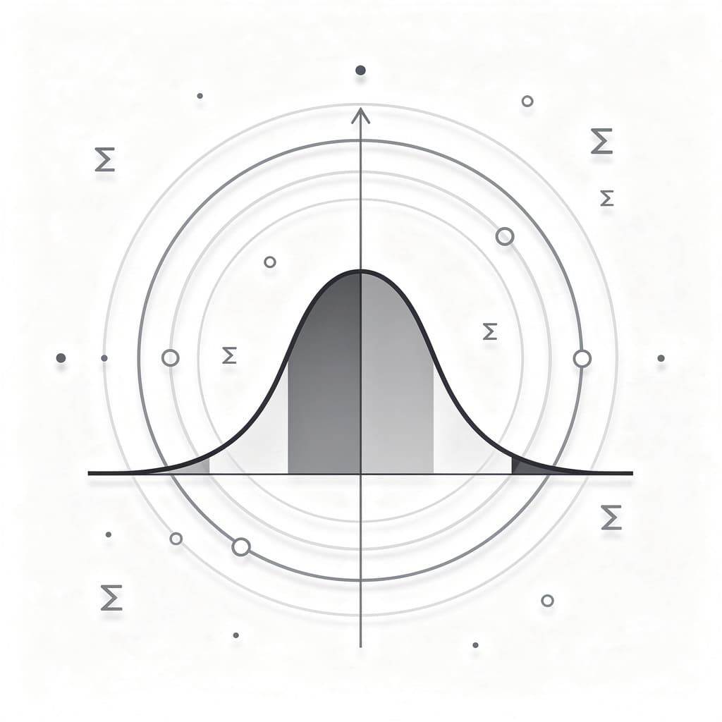
The relationship between standard deviation and the Normal Distribution, or the "bell curve," provides some of the most powerful predictive capabilities in statistics. For data that follows a normal distribution, the Empirical Rule (also known as the 68-95-99.7 rule) states that approximately 68% of all data points will fall within one standard deviation of the mean. This percentage increases to 95% within two standard deviations and a staggering 99.7% within three standard deviations. This mathematical certainty allows researchers to predict the probability of future events with remarkable accuracy. If you know the mean and standard deviation of human heights, you can calculate exactly how rare it is to find someone over seven feet tall.

Understanding Z-scores is the next step in applying standard deviation to real-world comparisons. A Z-score represents the number of standard deviations a specific data point is from the mean. For example, if a student receives a score with a Z-score of +2.0, it means they performed better than approximately 97.5% of their peers. Z-scores allow us to compare apples to oranges; we can use them to determine whether a student is "smarter" in math or verbal reasoning by seeing which score sits more standard deviations above the average for each respective test. This process of standardization is what makes large-scale testing and comparative research possible across different fields and scales.

Finally, the shape of the distribution and the presence of outliers can be quickly assessed through the lens of standard deviation. In a perfectly symmetrical normal distribution, the mean, median, and mode are all located at the same point, and the standard deviation perfectly describes the width of the bell. However, in "skewed" distributions where data trails off to one side, the standard deviation may be pulled away from the bulk of the data by extreme outliers. Identifying points that lie more than three standard deviations from the mean is a common technique for detecting anomalies. Whether these outliers represent a miraculous breakthrough in a medical trial or a simple data entry error, the standard deviation provides the objective threshold needed to flag them for further scrutiny.