Understanding the Normal Distribution: Definition, Formula, and Examples

The normal distribution, often referred to as the Gaussian distribution, represents one of the most significant concepts in modern statistics and probability theory. It describes a continuous probability distribution where data points cluster around a central mean, creating a symmetrical, bell-shaped curve that tapers off toward the extremes. This mathematical model serves as a cornerstone for statistical inference because many natural phenomena, from human heights to measurement errors in scientific instruments, tend to follow this pattern. By providing a predictable framework for understanding variance, the normal distribution allows researchers to make precise calculations about the likelihood of specific outcomes within a population. Its ubiquity in both theoretical mathematics and applied sciences makes it an essential tool for data analysis and decision-making across diverse fields.

Foundations of the Normal Distribution and Probability Density Function

The Concept of Continuous Probability Distributions

In the study of statistics, variables are generally categorized as either discrete or continuous, and the normal distribution falls firmly into the latter category. While discrete distributions deal with countable outcomes, such as the number of heads in a series of coin flips, continuous distributions describe variables that can take on any value within a range, such as time, weight, or temperature. The transition from discrete to continuous models occurs when the intervals between possible values become infinitely small, necessitating a shift from simple summation to calculus-based integration. This conceptual leap allows mathematicians to model real-world data where measurements can be infinitely precise, providing a more accurate representation of natural variability. Consequently, the normal distribution serves as the limiting form for many other distributions as the sample size increases, a phenomenon fundamentally linked to the Law of Large Numbers.

The historical development of the normal distribution is often credited to Carl Friedrich Gauss, though its foundations were laid earlier by Abraham de Moivre. De Moivre first discovered the distribution as an approximation to the binomial distribution when the number of trials is large, simplifying complex calculations for gamblers and astronomers alike. However, it was Gauss who popularized its use in the early 19th century to describe the distribution of errors in astronomical observations, leading to the term "Gaussian distribution." This historical context highlights the distribution's origins as a practical solution to measurement uncertainty rather than a purely abstract mathematical curiosity. Today, this foundation supports the vast majority of parametric statistical tests used in academic and industrial research.

Defining the Probability Density Function

The probability density function (PDF) is the mathematical rule that defines the shape and behavior of a continuous distribution. Unlike discrete distributions, where the function provides the probability of a specific point, the PDF for a normal distribution describes the relative likelihood of a random variable falling within a particular range. The value of the PDF at any given point $x$ does not represent a probability itself, as the probability of a continuous variable hitting an exact, single value is technically zero. Instead, the probability is found by calculating the area under the curve between two defined points on the horizontal axis. This distinction is vital for understanding why the height of the bell curve reflects density rather than discrete chance.

Mathematically, the PDF ensures that the total area under the curve is always equal to one, representing a 100 percent cumulative probability. This normalization allows statisticians to compare different sets of data by looking at their relative density across the distribution's span. Because the function is defined for all real numbers from negative infinity to positive infinity, it theoretically accounts for all possible outcomes, no matter how extreme. In practice, the density drops so rapidly as one moves away from the center that values beyond a few standard deviations are considered negligible. This concentration of density near the center is what gives the distribution its characteristic predictive power.

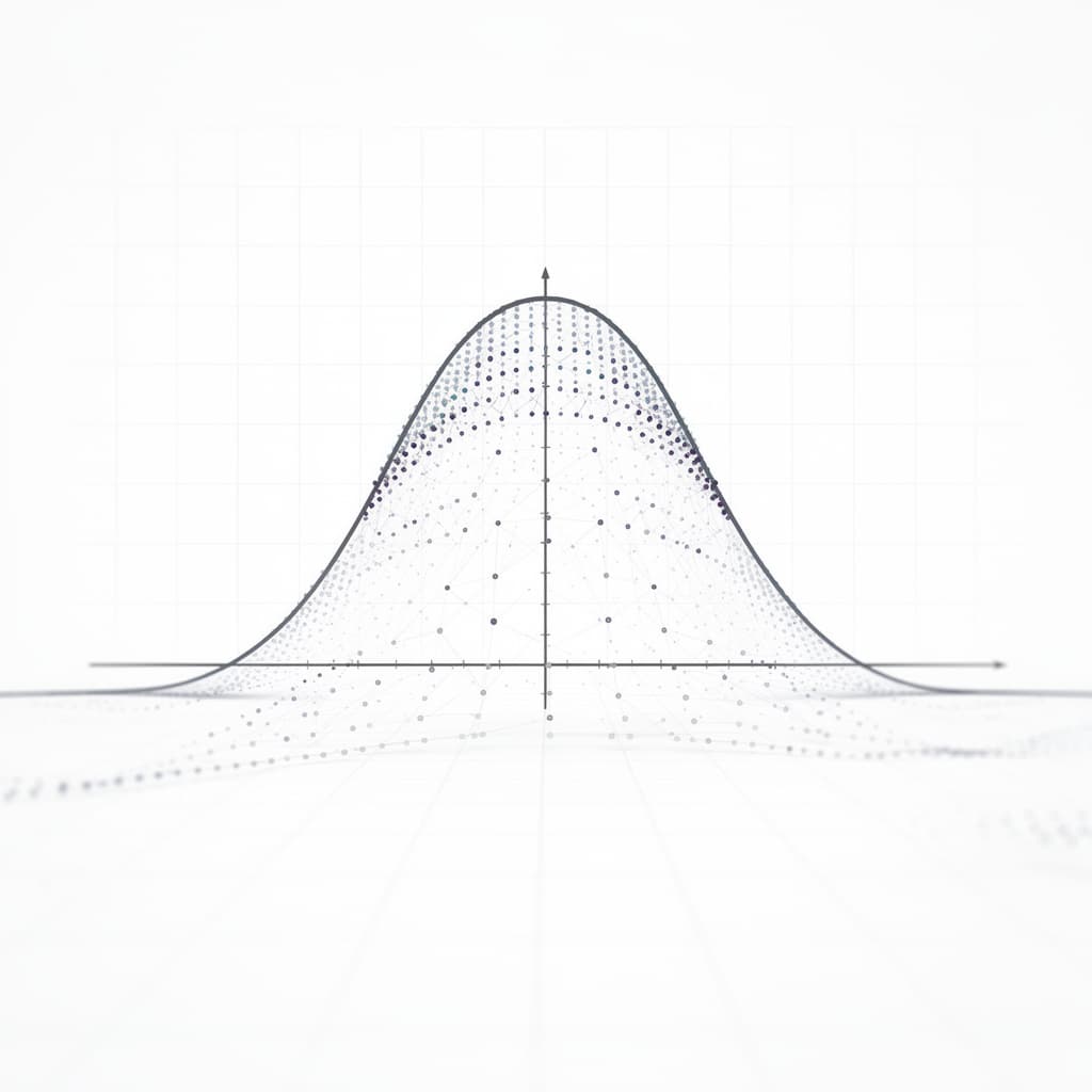
Visualizing the Symmetrical Bell Curve Shape

The visual representation of a normal distribution is famously known as the bell curve due to its distinctive rising peak and sloping sides. This shape is perfectly symmetrical, meaning that the left half of the distribution is a mirror image of the right half, centered exactly on the mean. The curve starts low on the horizontal axis, rises to a maximum height at the center, and then descends back toward the axis at an identical rate. This symmetry implies that values higher than the average are just as likely to occur as values lower than the average. This visual balance is not just an aesthetic feature but a fundamental property that simplifies many statistical calculations and interpretations.

As one moves away from the center, the curve exhibits a "tapering" effect, where the slope becomes less steep as it approaches the horizontal axis. These tapering ends are known as the tails of the distribution, and they represent the occurrence of extreme or rare events. In a true normal distribution, these tails are asymptotic, meaning they get closer and closer to the axis without ever actually touching it. This suggests that while extreme outliers are highly improbable, they are never mathematically impossible within the Gaussian framework. The relationship between the height of the peak and the width of the tails is determined entirely by the spread of the data, which defines the "flatness" or "sharpness" of the bell shape.

Mathematical Structure of the Bell Curve Formula

Breaking Down the Gaussian Equation

The mathematical foundation of the normal distribution is expressed through a specific equation that defines the height of the curve for any given value of $x$. This formula is essential for calculating probabilities and performing statistical modeling. The bell curve formula, or the Gaussian PDF, is defined as:

$$f(x | \mu, \sigma) = \frac{1}{\sigma \sqrt{2\pi}} e^{-\frac{(x - \mu)^2}{2\sigma^2}}$$

This equation contains several key mathematical constants and variables that determine the curve's behavior. The constant $\pi$ (approximately 3.14159) and the base of the natural logarithm $e$ (approximately 2.71828) are fundamental to the relationship between the curve's area and its exponential decay. The term $\frac{1}{\sigma \sqrt{2\pi}}$ acts as a normalization constant, ensuring that the total area under the curve integrates to exactly one regardless of the values chosen for the parameters. The exponent contains the square of the difference between the data point and the mean, which ensures that the result is always positive and that values further from the mean result in a smaller functional output.

Understanding the exponent is crucial for grasping how the curve creates its bell shape. The term $(x - \mu)^2$ measures the squared distance of a point from the center, and because it is negative in the exponent, larger distances result in smaller values for $f(x)$. This is why the curve is highest when $x = \mu$, as the exponent becomes zero and $e^0$ equals one. As $x$ moves away from $\mu$ in either direction, the value of the exponent decreases rapidly, causing the "drop" seen in the bell curve's tails. The presence of $\sigma^2$ (the variance) in the denominator of the exponent controls how quickly this drop occurs, effectively stretching or compressing the curve horizontally.

The Role of Mu and Sigma as Distribution Parameters

A specific normal distribution is entirely defined by two parameters: the mean ($\mu$) and the standard deviation ($\sigma$). The mean, denoted by the Greek letter mu, determines the location of the peak on the horizontal axis, serving as the center of gravity for the entire distribution. If the mean increases, the entire bell curve shifts to the right; if it decreases, the curve shifts to the left. However, changing the mean does not alter the shape or "spread" of the curve itself. In this sense, $\mu$ is a location parameter that tells us where the data is centered in the coordinate system.

The standard deviation, denoted by the Greek letter sigma, is the scale parameter that dictates the width and height of the distribution. A small $\sigma$ indicates that the data points are clustered closely around the mean, resulting in a tall, narrow bell curve with thin tails. Conversely, a large $\sigma$ signifies that the data is more spread out, leading to a shorter, wider curve with thicker tails. Because the total area must remain equal to one, any increase in width must be compensated by a decrease in the height of the peak. Together, $\mu$ and $\sigma$ allow statisticians to describe an infinite variety of normal distributions using just two numbers.

Calculation of the Mean, Median, and Mode

In a perfectly symmetrical normal distribution, the three primary measures of central tendency—the mean, median, and mode—are all exactly equal and located at the center of the curve. The mean is the arithmetic average of all data points, the median is the middle value that splits the data into two equal halves, and the mode is the most frequently occurring value. Because the highest point of the bell curve occurs at $x = \mu$, the mode is clearly at the center. Furthermore, because the curve is symmetrical, exactly 50 percent of the area lies to the left of the mean and 50 percent to the right, which satisfies the definition of the median.

This convergence of central measures is a defining characteristic of normality. In many other types of distributions, such as skewed distributions, these three values diverge significantly, with the mean being pulled toward the long tail. For example, in a right-skewed distribution, the mean is typically greater than the median, which is greater than the mode. The fact that $\text{Mean} = \text{Median} = \text{Mode}$ in a normal distribution simplifies data interpretation, as any of these measures can be used to represent the "typical" value of the set. When researchers find that a sample's mean and median are nearly identical, it is often used as a preliminary indicator that the data may follow a normal distribution.

Key Normal Distribution Properties and Characteristics

Total Area Under the Curve Calculation

One of the most important normal distribution properties is that the total area under the probability density function is always equal to exactly one. This property is a requirement for any valid probability distribution, as it represents the certainty that the random variable will take on some value within the set of all possible real numbers. Mathematically, this is expressed through the definite integral of the Gaussian function from negative infinity to positive infinity. Even though the curve extends forever in both directions, the exponential decay is so powerful that the area converges to a finite value. This allows us to interpret sub-areas of the curve as specific probabilities for ranges of data.

To calculate the probability that a value falls between two points $a$ and $b$, one must find the area under the curve between those two points. This is represented by the integral: $$P(a < X < b) = \int_{a}^{b} \frac{1}{\sigma \sqrt{2\pi}} e^{-\frac{(x - \mu)^2}{2\sigma^2}} dx$$ Since there is no closed-form algebraic solution (indefinite integral) for this function, these probabilities are typically determined using numerical integration, software packages, or standardized lookup tables. The concept of the "area as probability" is the foundation for almost all statistical testing, including the calculation of p-values and confidence intervals.

Symmetry and Asymptotic Convergence to the Axis

The symmetry of the normal distribution is absolute, meaning the skewness of the distribution is exactly zero. For every point $x = \mu + d$, the value of the PDF is identical to the value at $x = \mu - d$. This symmetry makes it easy to calculate probabilities for one half of the distribution and apply them to the other. For instance, if you know the probability of a value being more than two standard deviations above the mean, you automatically know the probability of a value being more than two standard deviations below the mean. This balance reflects many natural systems where deviations from the average are equally likely in both directions.

Asymptotic convergence refers to the way the tails of the curve approach the x-axis. No matter how far you travel from the mean, the value of $f(x)$ will be greater than zero, though it becomes astronomically small very quickly. This implies that the range of a normal distribution is technically infinite, $(-\infty, \infty)$. While this might seem counterintuitive for physical measurements like height (which cannot be negative), the probability of such values in a correctly modeled normal distribution is so low that they are effectively zero for practical purposes. This mathematical "openness" ensures that the model remains flexible enough to account for even the most extreme outliers imaginable.

Inflection Points and Standard Deviation

The shape of the bell curve changes from being "concave down" at the peak to "concave up" as it moves into the tails. The specific points where this change in curvature occurs are known as inflection points. In a normal distribution, these inflection points occur exactly at one standard deviation away from the mean, specifically at $x = \mu - \sigma$ and $x = \mu + \sigma$. This geometric property provides a visual way to estimate the standard deviation of a distribution just by looking at its graph. If you can identify where the curve stops "cupping" the mean and starts "flattening" toward the axis, you have found the distance of one $\sigma$.

The relationship between the inflection points and the standard deviation is fundamental to the "width" of the curve. Because $\sigma$ is the distance from the mean to the inflection point, it serves as a natural unit of measurement for the distribution. A larger $\sigma$ pushes these inflection points further from the center, creating a broader, gentler slope. A smaller $\sigma$ pulls them inward, creating a sharp, steep peak. This consistency across all normal distributions is what allows for the creation of the Empirical Rule, as the proportion of the area contained between these inflection points is always the same, regardless of the specific values of $\mu$ and $\sigma$.

Understanding the Empirical Rule 68-95-99.7

Data Distribution Within One Standard Deviation

The empirical rule 68-95-99.7, also known as the Three-Sigma Rule, is a shorthand used to remember the percentage of data that falls within specific ranges of a normal distribution. The first part of the rule states that approximately 68.27% of all observations will fall within one standard deviation of the mean ($\mu \pm 1\sigma$). This means that in a normally distributed population, more than two-thirds of the data points are relatively close to the average. For example, if the average height of a group is 170 cm with a standard deviation of 10 cm, roughly 68% of the people will be between 160 cm and 180 cm tall. This concentration of data near the center is the primary reason why the "average" is so representative of the group in Gaussian models.

From a practical standpoint, this 68% interval serves as the "typical" range for a dataset. In many industrial and scientific applications, values within this range are considered standard or expected. When monitoring a process, if a data point falls outside this range, it is not necessarily unusual, but it does indicate that the value is moving away from the most common central cluster. Understanding this first tier of the empirical rule helps researchers quickly gauge the density of their data and identify how much "churn" or variation exists near the mean before looking at more extreme outcomes.

The 95 Percent Interval for Statistical Significance

The second tier of the empirical rule states that approximately 95.45% (often rounded to 95%) of the data falls within two standard deviations of the mean ($\mu \pm 2\sigma$). This range is critically important in the world of statistics because the 95% threshold is the standard benchmark for determining "statistical significance." If a value falls outside of this range—meaning it is in the upper or lower 2.5% of the tails—it is often considered "unusual" or "statistically significant" at the alpha = 0.05 level. Using the previous height example, 95% of the population would fall between 150 cm and 190 cm (170 $\pm$ 20 cm).

The 95% interval is frequently used to construct confidence intervals in polls and scientific studies. When a researcher says they are "95% confident" that a value lies within a certain range, they are essentially invoking this property of the normal distribution. This boundary helps separate random noise from meaningful patterns; if an experimental result falls into the outer 5% of the distribution, it suggests that the result is unlikely to have occurred by chance alone. Consequently, the $\mu \pm 2\sigma$ range is perhaps the most frequently cited interval in applied data science and social research.

Rare Events and the Outer 99.7 Percent Boundary

The final tier of the empirical rule specifies that 99.73% of the data falls within three standard deviations of the mean ($\mu \pm 3\sigma$). This covers almost the entire area under the curve, leaving only 0.27% of the data to fall in the extreme tails (about 1 in 370 observations). Events that occur beyond this three-sigma boundary are considered extremely rare or "outliers." In manufacturing, the "Six Sigma" methodology is based on this principle, aiming to keep process variations so tight that defects (points falling outside the required range) occur at a rate of only a few per million, which is even more stringent than the three-sigma limit.

Understanding the 99.7% boundary is vital for risk management and quality control. In finance, for example, a "Black Swan" event is often described as a data point that falls many standard deviations away from the mean—an event so rare that the normal distribution suggests it should almost never happen. When data points frequently appear beyond the $3\sigma$ mark, it is a strong signal that the underlying population may not actually be normally distributed, or that the process has become unstable. This rule allows for the creation of control charts where any point exceeding the $3\sigma$ line triggers an immediate investigation into the cause of the variation.

The Standard Normal Distribution and Z-Score Calculation

Converting Raw Data into Standardized Z-Scores

While there are infinite possible normal distributions, they can all be related to a single baseline through the process of standardization. A z-score calculation transforms a raw data point $x$ into a value that represents how many standard deviations it is away from the mean. This allows for the comparison of data points from different distributions that have different means and scales. For instance, a z-score can help determine whether a specific score on a math test (mean 70) is better than a specific score on a history test (mean 50) by putting them on a common scale. The formula for calculating a z-score is:

$$z = \frac{x - \mu}{\sigma}$$

A positive z-score indicates that the data point is above the mean, while a negative z-score indicates it is below the mean. A z-score of 0 means the point is exactly at the mean. By converting data into z-scores, we effectively "center" the distribution at zero and "rescale" the width so that the standard deviation is one. This standardization process is a prerequisite for many advanced statistical techniques, including regression and factor analysis, as it ensures that variables with different units (like kilograms vs. meters) can be analyzed together fairly.

The Properties of the Unit Normal Curve

The standard normal distribution, often called the unit normal curve, is a special case of the normal distribution where the mean $\mu = 0$ and the standard deviation $\sigma = 1$. It is denoted as $Z \sim N(0, 1)$. Because every normal distribution can be mapped to this standard form, it serves as the universal reference for statistical tables. The probability density function for the standard normal distribution simplifies significantly because $\mu$ drops out and $\sigma$ becomes 1. This standardized version allows mathematicians to pre-calculate the areas under the curve once and apply those values to any normal distribution in existence.

The unit normal curve is perfectly symmetrical around zero. Its inflection points are at $z = 1$ and $z = -1$. The total area remains 1, and the empirical rule percentages (68, 95, 99.7) apply directly to the z-values of 1, 2, and 3. Most introductory statistics courses focus heavily on the unit normal curve because it teaches students how to think about relative position rather than absolute values. Once a student masters the unit normal curve, they can solve probability problems for any normally distributed variable by simply converting the raw values into z-scores first.

Using Z-Tables to Determine Probability

Before the ubiquity of high-powered computers and statistical software, the standard normal distribution was utilized primarily through z-tables. A z-table is a pre-calculated matrix of values that provides the cumulative probability (the area to the left) for a given z-score. To use the table, a researcher calculates the z-score for their data point, finds the corresponding row and column in the table, and retrieves the decimal value representing the probability. For example, a z-score of 1.96 corresponds to a cumulative probability of approximately 0.975, meaning 97.5% of the data falls below that point.

The table below illustrates a few common z-scores and their corresponding cumulative probabilities, which are foundational for understanding the distribution of data.

Z-Score ($z$)	Cumulative Probability ($P(Z < z)$)	Description
-3.0	0.0013	The extreme lower tail (0.13%)
-1.96	0.0250	Lower bound for 95% confidence
0.0	0.5000	The exact mean/median
1.0	0.8413	Mean plus one standard deviation
1.96	0.9750	Upper bound for 95% confidence
3.0	0.9987	The extreme upper tail (99.87%)

In modern practice, software functions like norm.dist() in Excel or scipy.stats.norm.cdf() in Python have replaced physical tables. However, the logic remains the same: the computer is numerically integrating the Gaussian formula to find the area under the curve. Whether using a table or a computer, the goal is to determine where a specific observation sits within the broader context of the population's variance.

Real-World Examples of Normal Distributions in Nature

Biological Measurements in Human Populations

One of the most classic examples of the normal distribution in the real world is the distribution of physical traits within a biological species. Human height, for instance, is almost perfectly normally distributed. If you were to measure every adult male in a large city and plot the results, you would see a clear bell curve centered around the average height (approx. 177 cm or 5'10" in many regions). Most men would be within a few inches of that average, with fewer and fewer men appearing as you look toward the very short or very tall ends of the spectrum. This occurs because height is a polygenic trait, meaning it is influenced by the additive effects of many different genes and environmental factors, which naturally tends toward a Gaussian distribution.

Similarly, intelligence quotient (IQ) scores are designed to follow a normal distribution by construction. The mean IQ is set at 100 with a standard deviation of 15. This means that about 68% of the population has an IQ between 85 and 115, and about 95% falls between 70 and 130. By forcing these scores into a normal distribution, psychologists can easily categorize individuals based on their relative standing. A score of 145, for example, is three standard deviations above the mean ($z = 3$), identifying it as an extremely rare event occurring in only 0.1% of the population. These biological and psychometric applications demonstrate how the normal distribution helps us define what is "typical" and "extraordinary" in nature.

Errors in Measurement and Scientific Data

In the physical sciences, the normal distribution is frequently used to model the "noise" or error associated with experimental measurements. When a scientist measures the mass of a chemical sample or the speed of light, no single measurement is perfectly accurate due to a multitude of tiny, uncontrollable factors. These factors—such as fluctuations in temperature, mechanical vibrations, or human reaction time—act as independent random variables. According to the Central Limit Theorem, the sum of these small, independent errors will follow a normal distribution. This is why repeated measurements of the same physical constant tend to cluster around the true value in a bell shape.

Gauss originally utilized this property to improve the accuracy of astronomical charts. He realized that by assuming errors were normally distributed, he could use the method of least squares to find the most probable location of a celestial body. In modern laboratories, this same principle is used to report "margin of error." When a result is given as $10.5 \pm 0.2$ grams, the scientist is often implying that the measurement follows a normal distribution where the standard deviation of the error is 0.2. This allow other researchers to understand the precision of the work and the likelihood that the true value falls within a certain range of the reported measurement.

Quality Control Variance in Manufacturing Processes

The world of industrial manufacturing relies heavily on the normal distribution to ensure product consistency and safety. When a machine fills soda bottles or cuts steel bolts, there is always a slight variation in the output. If the machine is functioning correctly, these variations are small and normally distributed around the target value. Quality control engineers monitor this variance by taking periodic samples and plotting them on control charts. If the distribution starts to shift (changing $\mu$) or spread out (changing $\sigma$), it indicates that the machine needs maintenance or that the process has been compromised by an external factor.

This application is best exemplified by the "Six Sigma" quality management strategy. In a Six Sigma process, the goal is to make the manufacturing so precise that the distance from the mean to the nearest specification limit (the point where a product is considered defective) is at least six standard deviations. Under this model, even if the mean shifts slightly, the probability of producing a defective part remains incredibly low—approximately 3.4 defects per million opportunities. This rigorous application of the normal distribution’s properties allows modern industry to produce complex electronics and safety-critical aerospace components with near-perfect reliability, proving that the bell curve is much more than just a mathematical abstraction; it is a vital tool for the modern world.