The Elegant Logic of Statistical Dispersion

Statistical dispersion represents the fundamental measure of how "spread out" a dataset is, providing the necessary context that central tendency measures like the mean often omit. While the arithmetic mean offers a snapshot of the average value, it remains silent regarding the volatility or consistency of the underlying data points. Statistical dispersion, particularly through the lens of variance and standard deviation, allows researchers to quantify the reliability of their averages and understand the diversity within a population. By mastering how to calculate standard deviation, one gains the ability to discern whether a mean is a representative anchor or a misleading artifact of extreme outliers.

Defining Dispersion and Central Tendency

To appreciate the elegance of statistical dispersion, one must first recognize the inherent limitations of central tendency. Imagine two cities with an identical average annual temperature of 20 degrees Celsius; in the first city, the temperature remains a steady 20 degrees year-round, while the second fluctuates between negative 10 and 50 degrees. Without a measure of dispersion, a traveler would mistakenly assume both climates offer the same experience. Dispersion provides the "elbow room" around the mean, describing the extent to which data points stretch, squeeze, or cluster. It is the bridge between a simple summary and a comprehensive understanding of a dataset’s architecture.

Measuring the deviation from the mean is the primary method through which we quantify this spread. A deviation is simply the distance between a specific data point and the average of the entire set. If we merely summed these distances, the positive and negative values would cancel each other out, resulting in a sum of zero regardless of how much the data varied. To circumvent this mathematical vanishing act, statisticians developed methods to treat all distances as positive quantities, ensuring that every piece of variability contributes to the final metric. This pursuit of a "mean distance" from the center is what leads us directly into the mathematical territory of variance and its square root.

The concept of variability is not merely a mathematical abstraction but a reflection of the natural world’s unpredictability. Whether measuring the heights of biological organisms, the return on financial investments, or the precision of industrial components, variability is the noise that analysts seek to tame. By formalizing this noise into a single number, we can compare the stability of different systems. Statistical dispersion thus serves as a proxy for risk, uncertainty, and diversity, allowing for a more nuanced interpretation of data that goes far beyond the simplistic "typical" value suggested by the mean.

Mathematical Foundations of Variance

Variance serves as the squared foundation of modern dispersion metrics, born from the need to eliminate the directionality of data points. When calculating the distance of a point $x_i$ from the mean $\mu$, the resulting value $(x_i - \mu)$ can be negative if the point is below the average. By squaring the differences, we ensure that every deviation—whether above or below the mean—contributes a positive value to our measure of spread. This mathematical transformation is known as the "sum of squares," and it forms the numerator of the variance formula. Squaring also has the side effect of disproportionately weighting larger deviations, which makes variance highly sensitive to outliers.

While squaring the differences solves the problem of negative numbers, it introduces a significant conceptual hurdle: the problem of squared units. If a dataset measures the weight of apples in grams, the variance of that dataset is expressed in "square grams." This unit shift makes the variance difficult to visualize or compare directly with the original data. For instance, stating that the variance of a group’s height is 400 square centimeters is far less intuitive than stating their heights vary by a certain number of centimeters. Understanding the variance vs standard deviation relationship requires recognizing that variance is an intermediate step—a calculation that captures total variability before we return to the original scale.

The transition from variance to standard deviation is achieved by taking the square root of the variance. This operation effectively "undoes" the squaring process, bringing the measure of dispersion back into the same units as the original observations. If the variance is denoted as $\sigma^2$ for a population, then the standard deviation is $\sigma$. This relationship is not merely a convenience of units; it is a mathematical necessity for many advanced statistical distributions. Variance remains the workhorse of theoretical statistics because squared terms are easier to manipulate in calculus, but standard deviation remains the preferred choice for reporting and interpretation due to its physical groundedness.

How to Calculate Standard Deviation

Learning how to calculate standard deviation involves a systematic approach that transforms a raw list of numbers into a single, descriptive parameter. The process begins with the standard deviation formula, which for a population is expressed as:

$$\sigma = \sqrt{\frac{\sum_{i=1}^{N} (x_i - \mu)^2}{N}}$$

In this formula, $\sigma$ represents the population standard deviation, $x_i$ is each individual value, $\mu$ is the population mean, and $N$ is the total number of observations. The $\sum$ (sigma) symbol dictates that we must sum the squared differences for every single point in the set before dividing by the count. This formula essentially computes the "root-mean-square" of the deviations, providing a quadratic average of how much the values deviate from the center.

To execute a standard deviation step by step calculation, one should follow a rigid five-step sequence to avoid common errors. First, find the arithmetic mean ($\mu$) by summing all data points and dividing by the count ($N$). Second, subtract the mean from each individual data point to find the deviation of each point. Third, square each of those resulting deviations to make them positive. Fourth, calculate the average of these squared deviations (which is the variance). Finally, take the square root of that average to arrive at the standard deviation. This sequence ensures that the final number accurately reflects the "typical" distance from the mean.

Let us consider a concrete example using a small dataset of test scores: 70, 80, and 90. The mean score is 80. The deviations are $-10$ ($70-80$), $0$ ($80-80$), and $10$ ($90-80$). Squaring these deviations gives us 100, 0, and 100. The sum of these squares is 200. Dividing by the number of scores ($N=3$) gives a variance of approximately 66.67. Taking the square root of 66.67 results in a standard deviation of approximately 8.16. This number tells us that, on average, the scores in this set deviate from the mean of 80 by about 8.16 points, providing a clear metric for the group's performance consistency.

Population vs Sample Standard Deviation

A critical distinction in statistics arises from the source of the data: whether it encompasses the entire population or merely a representative sample. When calculating the dispersion for an entire population, we use $N$ in the denominator. However, when working with a sample, we employ Bessel's correction, which involves dividing by $n - 1$ instead of $n$. This adjustment accounts for the fact that a sample is likely to be slightly less diverse than the full population it represents. By reducing the denominator, we slightly increase the resulting standard deviation, which serves to correct the inherent bias that causes samples to underestimate the true population variance.

The logic behind $n - 1$, often referred to as "degrees of freedom," is rooted in the constraint that the sum of deviations from the mean must always equal zero. If we know the mean and $n - 1$ of the data points, the last data point is "fixed" and not free to vary. Therefore, only $n - 1$ pieces of information are truly independent when estimating the population variance from a sample. This correction was popularized by the mathematician Friedrich Bessel and remains a cornerstone of frequentist statistics. Failing to use this correction in inferential statistics can lead to overly optimistic conclusions about the precision of an estimate.

Selecting the correct parameter is a matter of defining the scope of the study. If a teacher calculates the grades for their specific class to describe that class alone, they are calculating the population standard deviation for that specific group. However, if that teacher uses those same grades to estimate the variability of grades across the entire school district, they must treat the class as a sample and use $n - 1$. This distinction between population vs sample standard deviation is the difference between descriptive statistics, which summarize what is observed, and inferential statistics, which predict what is unobserved.

Interpreting the Empirical Rule

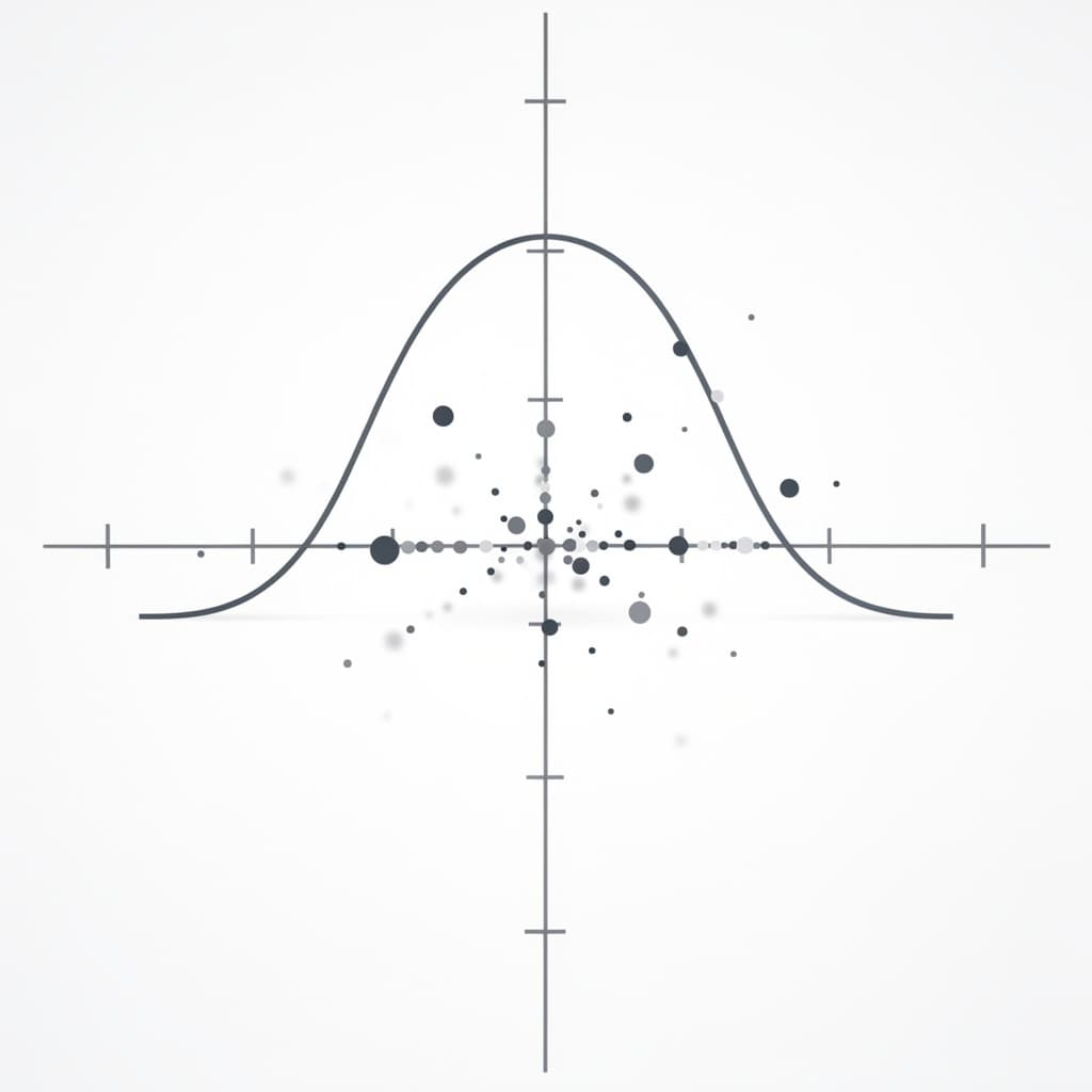
The true power of standard deviation is revealed when applied to the Normal Distribution, also known as the Gaussian curve or bell curve. In a perfectly symmetrical distribution, the empirical rule (or the 68-95-99.7 rule) provides a predictable framework for understanding data density. Approximately 68 percent of all data points fall within one standard deviation ($\pm 1\sigma$) of the mean. This means that if you know the mean and the standard deviation of a normally distributed set, you can immediately identify where the vast majority of your observations reside without looking at the raw data.

As we move further from the center, the percentage of data accounted for increases significantly. Roughly 95 percent of data points fall within two standard deviations ($\pm 2\sigma$), and 99.7 percent fall within three standard deviations ($\pm 3\sigma$). This mathematical regularity allows statisticians to define what constitutes a "normal" range and what should be flagged as an anomaly. Any data point that falls beyond the $3\sigma$ threshold is often considered a statistical outlier, as the probability of such an occurrence happening by chance is less than 0.3 percent in a normal distribution.

Identifying outliers through sigma levels is a standard practice in fields ranging from medical research to manufacturing. For example, in a clinical trial, if a patient’s reaction time is four standard deviations away from the mean, researchers might investigate whether that patient represents a unique sub-population or if there was an error in measurement. The empirical rule transforms the standard deviation from a dry calculation into a diagnostic tool. It provides a universal language for "unusualness," allowing a scientist in Tokyo and a financier in New York to agree on exactly how extreme a particular event truly is.

Advanced Applications of Dispersion Logic

In the world of finance, the logic of dispersion is synonymous with the concept of risk. Portfolio managers use standard deviation to measure the volatility of an asset's returns over time. An investment with a high standard deviation is considered "risky" because its future value is highly uncertain and can deviate significantly from its expected mean return. The Sharpe Ratio, a fundamental tool for investors, uses standard deviation in its denominator to calculate how much excess return an investor receives for the extra volatility they endure. In this context, minimizing dispersion while maximizing the mean is the ultimate goal of rational wealth management.

Engineering and manufacturing rely heavily on dispersion logic through the lens of quality control, most notably in the Six Sigma methodology. Developed by Motorola in the 1980s, Six Sigma aims for a level of precision where the nearest "specification limit" (the point where a product becomes defective) is at least six standard deviations away from the mean of the production process. This translates to a failure rate of just 3.4 defects per million opportunities. By focusing on reducing the standard deviation of manufacturing processes, engineers ensure that even the "widest" outliers in production still result in functional, high-quality products.

Beyond these industries, the logic of standard deviation informs public policy, social sciences, and even artificial intelligence. In machine learning, dispersion is used in "regularization" techniques to prevent models from becoming overly sensitive to the noise in training data. In sociology, measuring the dispersion of income (often via the related Gini coefficient) tells a more complex story about a nation's health than GDP per capita alone. Whether we are looking at the micro-scale of subatomic particles or the macro-scale of global economics, the standard deviation remains the most robust and elegant tool for quantifying the inherent messiness of reality.

References

- Pearson, K., "Contributions to the Mathematical Theory of Evolution", Philosophical Transactions of the Royal Society of London, 1894.
- Bessel, F. W., "Untersuchungen über die Bahnen der Doppelsterne," Berlin Academy of Sciences, 1816.
- Fisher, R. A., "Statistical Methods for Research Workers", Oliver and Boyd, 1925.
- Stigler, S. M., "The History of Statistics: The Measurement of Uncertainty before 1900," Harvard University Press, 1986.
Recommended Readings
- The Lady Tasting Tea by David Salsburg — A fascinating narrative history of how statistics revolutionized science in the 20th century, making complex concepts like variance accessible.
- Against the Gods: The Remarkable Story of Risk by Peter L. Bernstein — This book explores the development of the concepts of probability and risk, showing how dispersion became the central pillar of modern finance.
- Standard Deviation: A Forgotten Legend of Social Science by Gary Smith — A deep dive into how standard deviation is misused and misunderstood in common discourse, offering a cautionary tale for data analysts.
- Naked Statistics by Charles Wheelan — An excellent primer that uses humor and real-world examples to build an intuitive grasp of statistical tools, including a stellar chapter on the logic of the bell curve.