The Statistical Logic of Standard Deviation

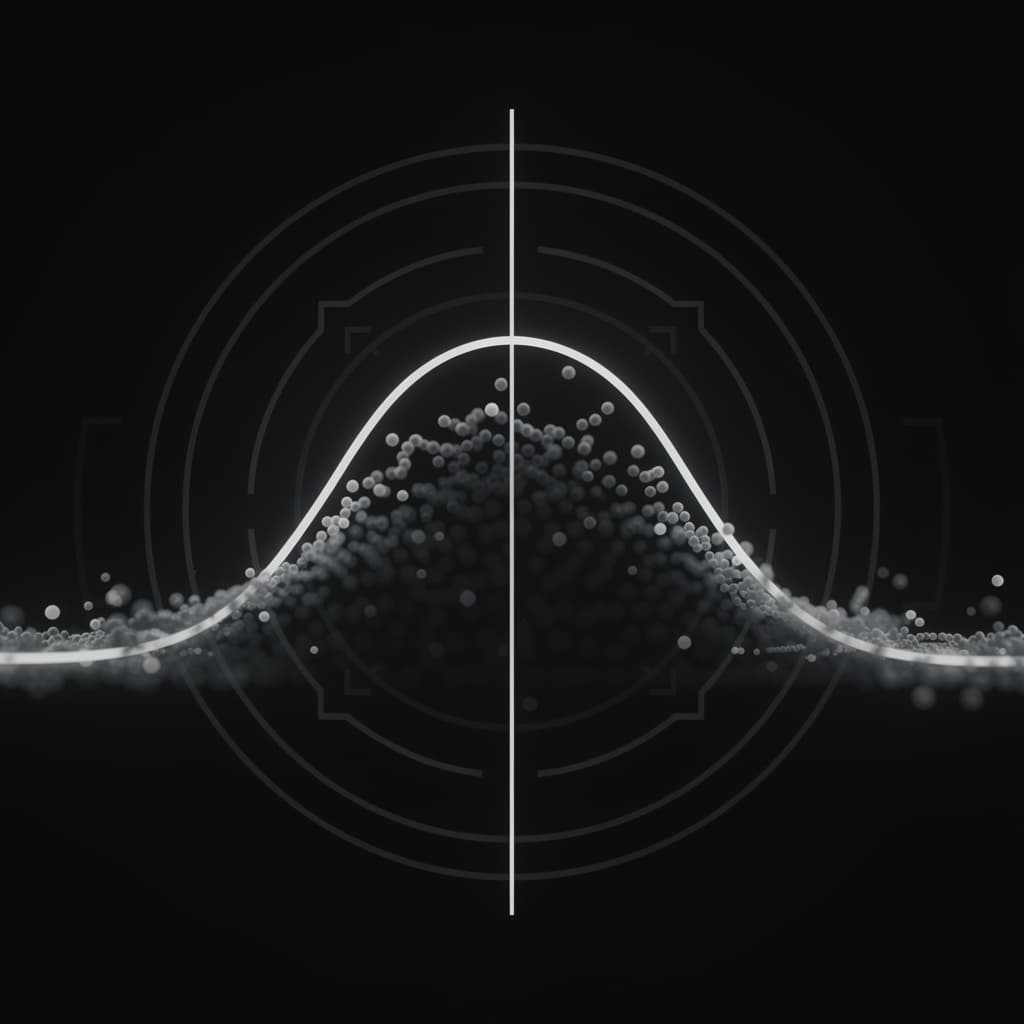
In the realm of descriptive statistics, the quest to summarize vast quantities of data often begins with measures of central tendency, such as the mean, median, and mode. However, knowing the average value of a dataset provides only a partial view of the underlying reality; it fails to describe how the individual data points are scattered around that center. The standard deviation serves as the most critical tool for quantifying this dispersion, offering a mathematically rigorous way to express the "typical" distance between a data point and the arithmetic mean. By transforming the concept of spread into a single, interpretable numerical value, standard deviation allows researchers, economists, and scientists to assess the reliability of their averages and the inherent volatility within their observations.

Defining the Measure of Dispersion

What is Standard Deviation in Statistics

In the broader context of statistical analysis, what is standard deviation but a measurement of the consistency or "tightness" of a dataset? When we observe a group of numbers, such as the heights of adults in a specific city, we expect some variation; the standard deviation provides a standardized metric to express that variation in the original units of measurement. A low standard deviation indicates that the data points tend to be very close to the mean, suggesting a high degree of uniformity and predictability within the sample. Conversely, a high standard deviation reveals that the data is spread out over a wider range of values, indicating greater diversity or, in many scientific contexts, greater uncertainty or risk.

The conceptual framework of standard deviation explained through daily examples often involves comparing two sets of data with the identical mean but vastly different characters. For instance, consider two climate zones where the average annual temperature is 20 degrees Celsius. In the first zone, the temperature rarely fluctuates more than five degrees from the mean, resulting in a low standard deviation and a stable climate. In the second zone, the temperature might swing between 0 and 40 degrees Celsius; despite sharing the same average, the high standard deviation signals an environment of extremes. This illustrates why the mean alone is insufficient for decision-making in fields ranging from agriculture to financial portfolio management.

The Relationship Between Mean and Variance

To understand standard deviation, one must first grasp the concept of variance, which is its mathematical predecessor. Variance is calculated by taking the average of the squared differences between each data point and the mean, providing a measure of spread that is strictly non-negative. While variance is computationally powerful—especially in the context of analysis of variance (ANOVA) and linear regression—it suffers from a lack of intuitive scale because its units are squared. If you are measuring the weight of livestock in kilograms, the variance would be expressed in "squared kilograms," a unit that holds no physical meaning in the real world.

The standard deviation solves this problem of interpretability by taking the square root of the variance, effectively returning the measure of spread to the original units of the data. This relationship ensures that the standard deviation is always in the same "language" as the mean, allowing for direct comparisons and the construction of confidence intervals. Mathematically, if variance is denoted as ${\sigma }^2$ for a population, the standard deviation is simply $\sigma$. This symbiotic relationship allows statisticians to use variance for algebraic manipulations and standard deviation for reporting results and visualizing the distribution of observations in a way that resonates with human intuition.

Breaking Down the Standard Deviation Formula

Components of the Mathematical Expression

The standard deviation formula may appear daunting at first glance, but it is a logical sequence of operations designed to capture the essence of variability. For a population, the formula is expressed as:

$$\sigma =\sqrt{\frac{{\sum }_{i=1}^N(x_i-\mu {)}^2}{N}}$$

In this expression, $\sigma$ (sigma) represents the population standard deviation, $\sum$ (sigma) denotes the summation symbol, $x_i$ represents each individual value in the dataset, and $\mu$ (mu) is the population mean. The denominator $N$ represents the total number of observations in the population. Each component plays a specific role: the term $(x_i-\mu )$ captures the "deviation" of each point, while the squaring and subsequent averaging distribute these deviations across the entire dataset to find a representative value.

When dealing with a sample rather than an entire population, the formula undergoes a slight but significant modification. The sample standard deviation, denoted by $s$, uses the sample mean $\bar{x}$ and a divisor of $n-1$ instead of $N$. This denominator change is known as Bessel’s correction, which accounts for the fact that a small sample is less likely to capture the extreme values of a population, potentially underestimating the true spread. By dividing by a slightly smaller number, the formula produces a slightly larger (and more accurate) estimate of the population’s variability, ensuring that the sample statistic remains an unbiased estimator of the population parameter.

Squared Deviations and the Role of the Square Root

A common question among students is why we square the deviations instead of simply taking the average of the absolute differences from the mean. The primary reason is mathematical: squaring the differences $(x_i-\mu )$ ensures that all values are positive, preventing negative deviations from cancelling out positive ones, which would result in a sum of zero. Furthermore, squaring emphasizes larger deviations, meaning that outliers have a disproportionately large impact on the final standard deviation. This sensitivity is often desirable in fields like engineering or quality control, where a single large error is much more significant than many small ones.

The final application of the square root is the "corrective" step that brings the measure back to a linear scale. Without the square root, we would be left with variance, which grows quadratically and obscures the relationship between the spread and the center of the data. By taking the square root, we align the standard deviation with the mean, creating a metric that can be added to or subtracted from the mean to define ranges. This alignment is what allows us to say, for example, that a certain value is "two standard deviations above the mean," a statement that provides immediate context regarding how unusual that value is relative to the rest of the group.

How to Calculate Standard Deviation Manually

Calculating the Arithmetic Mean

The first step in learning how to calculate standard deviation is the precise determination of the arithmetic mean. To find the mean, one must sum all individual observations in the dataset and divide that total by the number of observations ($N$ for population or $n$ for sample). For example, if we are analyzing the test scores of five students—80, 85, 90, 95, and 100—we first add these values to get a sum of 450. Dividing 450 by 5 yields a mean ($\mu$ or $\bar{x}$) of 90. This mean serves as the anchor point for all subsequent calculations, representing the center of gravity for the data distribution.

It is essential to ensure that the mean is calculated with high precision, as any rounding error at this stage will propagate through the squaring process and lead to an inaccurate final result. In professional scientific reporting, the mean is often calculated to several decimal places beyond the original data. Once the mean is established, the next sub-step involves subtracting this mean from every individual data point in the set. In our example, the deviations would be -10, -5, 0, 5, and 10; notice how these values sum to zero, illustrating why we cannot simply average the deviations themselves to measure spread.

Summing the Squares and Final Averaging

After determining the individual deviations, the next phase of how to calculate standard deviation involves squaring each of those differences. Squaring the deviations from our previous example gives us 100, 25, 0, 25, and 100. Summing these squared values produces a total of 250, which is technically referred to as the "sum of squares." This value represents the total aggregate variation present in the dataset, but it is not yet "standardized" because it depends on the number of data points. To normalize this value, we divide by the appropriate divisor: for a population, we divide by 5 (resulting in 50), or for a sample, we divide by $5-1=4$ (resulting in 62.5).

The final step is to take the square root of this average. If we were treating our student scores as a population, the square root of 50 is approximately 7.07. If we were treating them as a sample, the square root of 62.5 is approximately 7.91. This final value—7.07 or 7.91—is the standard deviation, representing the average distance the students' scores fell from the mean of 90. By following these standard deviation calculator steps manually, one gains a deep appreciation for how the metric balances every data point's contribution to the overall picture of volatility.

Population vs Sample Standard Deviation

Degrees of Freedom and Bessel’s Correction

The distinction between population vs sample standard deviation is one of the most frequent sources of confusion for statistics students, yet it is rooted in a fundamental logical necessity. When we calculate the standard deviation of an entire population, we have access to every possible data point, meaning the mean we calculate is the true population mean. However, when we work with a sample, we are using the sample mean ($\bar{x}$) as an estimate for the population mean ($\mu$). Because the sample mean is calculated from the sample itself, the data points in that sample tend to be closer to $\bar{x}$ than they would be to the true, unknown $\mu$. This inherent bias makes the sample appear less variable than the population actually is.

To correct for this underestimation of variability, statisticians apply what is known as degrees of freedom. In a sample of $n$ observations, once the sample mean is known, only $n-1$ observations are free to vary; the last observation is effectively "fixed" to ensure the mean remains what it is. By dividing by $n-1$ instead of $n$, we mathematically compensate for the bias introduced by using an estimated mean. This adjustment, known as Bessel's Correction, ensures that if we were to take many samples and calculate their standard deviations, the average of those sample standard deviations would converge on the true population standard deviation.

Choosing the Correct Divisor for Your Dataset

Choosing between $N$ and $n-1$ depends entirely on the scope of your inquiry and the nature of your data collection. If your dataset encompasses every single member of the group you are studying—for example, the test scores of every student in a specific, small classroom—you are dealing with a population. In this case, you use $N$ because there is no uncertainty regarding the mean; you have the complete picture. Population standard deviation is common in descriptive statistics where the goal is simply to summarize the specific data at hand without making broader generalizations.

However, if your data is intended to represent a larger group—such as a survey of 1,000 voters used to predict the behavior of an entire nation—you must use the sample standard deviation formula with $n-1$. This is the standard in almost all experimental research, clinical trials, and quality assurance testing. Most statistical software and scientific calculators provide two different functions, often labeled as ${\sigma }_n$ and $s_{n-1}$ (or $\sigma$ and $s$). Misidentifying your data as a population when it is actually a sample can lead to overly optimistic results, where the variability of the system is understated, potentially leading to errors in risk assessment or hypothesis testing.

Standard Deviation Explained Through Data Distribution

The Empirical Rule in Normal Distributions

One of the most powerful applications of the standard deviation is its role in describing the Normal Distribution, often called the "Bell Curve." In a perfectly normal distribution, the data is symmetric around the mean, and the standard deviation provides a "yardstick" for the probability of any given value occurring. The Empirical Rule (or the 68-95-99.7 rule) states that approximately 68 percent of the data falls within one standard deviation of the mean ($\mu \pm \sigma$), 95 percent falls within two standard deviations ($\mu \pm 2\sigma$), and 99.7 percent falls within three standard deviations ($\mu \pm 3\sigma$).

This rule allows statisticians to identify outliers and determine the "normality" of a dataset with remarkable speed. If you are measuring the weight of cereal boxes on a production line and the mean is 500 grams with a standard deviation of 5 grams, you know that 95 percent of all boxes will weigh between 490 and 510 grams. If you find a box weighing 480 grams, it is four standard deviations away from the mean, making it a "four-sigma" event. Such an occurrence is statistically rare (less than 0.01 percent chance), suggesting that the machinery might be malfunctioning or that the process is out of control.

Interpreting High and Low Volatility

In the financial world, standard deviation is the primary metric for volatility, which serves as a proxy for risk. When an investment has a high standard deviation, its historical returns have swung wildly, suggesting that while there is a potential for high gains, there is an equally high probability of significant losses. Investors who are "risk-averse" generally seek assets with low standard deviations, such as government bonds, which offer steady, predictable returns. Conversely, "risk-tolerant" investors might look at high-standard-deviation assets like technology stocks or cryptocurrencies, where the wide spread of potential outcomes reflects the higher uncertainty of the underlying market.

Outside of finance, interpreting volatility is crucial in biological and social sciences. A low standard deviation in a clinical trial's results might indicate that a drug has a very consistent effect across a diverse population. In contrast, a high standard deviation in the same trial might suggest that the drug works very well for some people but not at all for others, prompting researchers to investigate genetic or environmental sub-factors. Understanding these swings in data helps move beyond the "average person" fallacy, recognizing that the "average" is often a poor representation of any single individual in a highly volatile system.

Standard Deviation Calculator Steps for Accuracy

Data Input and Handling Outliers

When using a digital tool or software to process large datasets, the standard deviation calculator steps usually begin with rigorous data cleaning. Before inputting values into a spreadsheet like Excel or a statistical package like R, it is vital to check for "dirty data," such as typos, missing values, or obvious recording errors. Standard deviation is highly sensitive to outliers because the formula involves squaring the deviations; a single value entered as "1000" instead of "100" will catastrophically inflate the result, leading to an inaccurate representation of the dataset's typical spread.

Effective data handling often involves visualizing the dataset using a box plot or a histogram before performing the calculation. If outliers are identified, the researcher must decide whether they are legitimate variations (like the wealth of a billionaire in a local neighborhood survey) or errors that should be excluded. If the outliers are legitimate but skew the results too heavily, some analysts prefer to report the Interquartile Range (IQR) alongside the standard deviation, as the IQR is more robust and less influenced by extreme values. Ensuring the integrity of the input data is the most important "step zero" in any calculation process.

Verification of Algorithmic Results

Modern standard deviation calculator steps often rely on built-in functions such as STDEV.S for samples or STDEV.P for populations in Microsoft Excel. While these tools are incredibly efficient, it is best practice to verify the results, especially when working on high-stakes projects. A simple way to verify an algorithmic result is to perform a manual calculation on a small subset of the data or to use a secondary software package to see if the outputs match. This cross-verification helps identify whether the software is applying Bessel’s correction appropriately for your specific use case.

Furthermore, one should be aware of the "precision limit" of the software being used. When dealing with extremely large numbers or datasets with very tiny variations, some algorithms can suffer from floating-point errors or catastrophic cancellation during the subtraction phase of the calculation. High-end statistical software like SAS or SPSS uses "two-pass" algorithms that calculate the mean in the first pass and the sum of squares in the second pass to minimize these rounding errors. For the average user, the most important verification step is ensuring that the correct formula (sample vs population) was selected in the software settings, as this is the most common point of human-error-induced inaccuracies.

The Geometric Intuition of Spread

Euclidean Distance in Multi-Dimensional Space

Beyond the algebraic manipulation of numbers, there is a profound geometric interpretation of standard deviation. If we view a dataset of $n$ values as a single point in an $n$-dimensional Euclidean space, and the mean of that dataset as another point in the same space, the standard deviation is closely related to the Euclidean distance between these two points. Specifically, the numerator of the variance (the sum of squared deviations) is the square of the distance between the vector of data points and the vector where every entry is the mean. This perspective transforms a statistical concept into a spatial one, where "spread" is literally the distance between what we observed and what we expected.

This geometric view is essential in fields like machine learning and pattern recognition. When an algorithm "clusters" data, it is essentially looking for groups with low internal standard deviation—points that are geographically close to each other in a multi-dimensional feature space. By understanding standard deviation as a distance, it becomes easier to visualize why the measure is always non-negative and why the "root-mean-square" approach is the most efficient way to summarize the magnitude of errors in a system. It connects the abstract world of probability to the tangible world of geometry and physics.

Root Mean Square as a Physical Analogy

The standard deviation is a specific application of a broader mathematical concept known as the Root Mean Square (RMS). In physics and electrical engineering, RMS is used to calculate the "effective" value of an alternating current (AC) or the average power of a wave. Just as the standard deviation provides a stable measure of a variable's "distance" from the mean, the RMS provides a stable measure of a fluctuating signal's "distance" from zero. This analogy is helpful because it explains why we use the square root: it "rectifies" the fluctuations into a single, usable magnitude that performs the same "work" as a steady-state value.

In mechanical systems, the standard deviation of vibrations can indicate the health of a machine. A motor that is perfectly balanced will have a very low standard deviation in its displacement over time. As bearings wear out or parts become misaligned, the standard deviation of the displacement increases, even if the "average" position of the motor remains the same. This physical manifestation of the standard deviation underscores its universality; it is not merely a tool for statisticians, but a fundamental law of nature that describes the noise, friction, and inherent variability present in every physical and social system in the universe.

References

- Pearson, K., "Contributions to the Mathematical Theory of Evolution", Philosophical Transactions of the Royal Society of London, 1894.
- Fisher, R. A., "Statistical Methods for Research Workers", Oliver and Boyd, 1925.
- Bland, J. M., and Altman, D. G., "Statistics Notes: Measurement Error", British Medical Journal, 1996.
- Stigler, S. M., "The History of Statistics: The Measurement of Uncertainty before 1900", Belknap Press of Harvard University Press, 1986.
Recommended Readings
- The Lady Tasting Tea by David Salsburg — A fascinating narrative history of how statistics revolutionized science in the 20th century, making complex concepts like standard deviation accessible through the stories of the people who discovered them.
- Statistics in Plain English by Timothy C. Urdan — This book excels at breaking down mathematical formulas into conversational language, ideal for readers who want to understand the logic behind the calculations without getting lost in dense notation.
- Thinking Fast and Slow by Daniel Kahneman — While primarily about psychology, this work provides deep insights into why humans are naturally poor at intuitive statistics and why rigorous measures like standard deviation are necessary to overcome cognitive biases.
- Standard Deviation: A Forgotten Statistic by various contributors in the Journal of Statistics Education — A deeper dive into the pedagogical challenges of teaching dispersion and the common misconceptions held by students and professionals alike.
Turn this topic into a full course
Noesis builds the syllabus, notes and tests for you, and you study them with a tutor that knows your material.