The Analytical Mechanics of Rates of Change

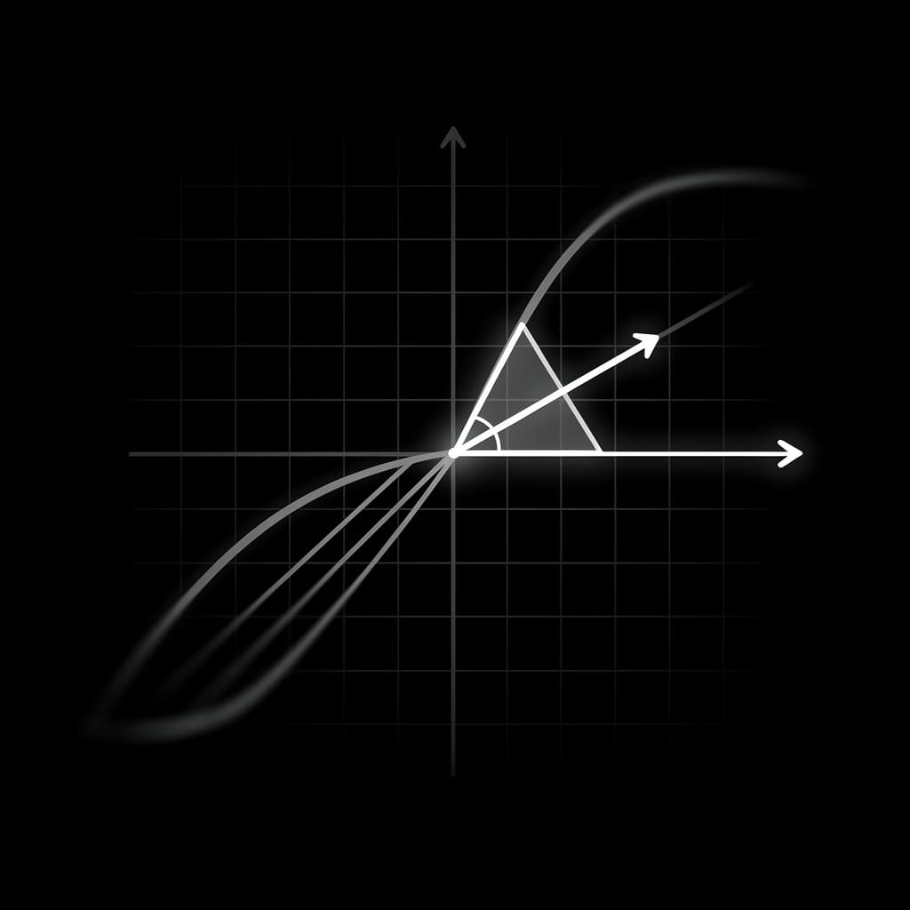
The study of analytical mechanics and the calculus of variations begins with a fundamental inquiry into the nature of change. In the static world of elementary algebra, variables represent fixed quantities, and relationships are expressed through linear equations that describe stable states. However, the physical universe is rarely static; it is defined by motion, growth, decay, and transformation. To understand these phenomena, mathematicians developed the concept of the derivative, a rigorous tool that quantifies the instantaneous rate of change of a function at any given point. By transitioning from the average slope of a line to the precise behavior of a curve at a single coordinate, analytical mechanics provides the framework for modern physics, engineering, and economics.

Foundations of Continuous Motion

The conceptual journey toward understanding how to find the derivative begins with the distinction between average and instantaneous rates of change. Consider a vehicle traveling between two cities: the average velocity is easily calculated by dividing the total distance by the total time. However, this average fails to describe the vehicle's speed at a specific moment in time, such as the exact second it passes a certain landmark. To capture this instantaneous rate of change, we must narrow the window of observation until the interval of time effectively approaches zero. This logical leap from a macroscopic average to a microscopic instant is the cornerstone of calculus, allowing us to define motion not just as a sequence of positions, but as a continuous flow.

Geometrically, this transition is visualized through the relationship between secant lines and tangent lines. A secant line connects two distinct points on a curve, representing the average slope over that interval. As the two points are moved closer together, the secant line begins to pivot, eventually settling into a position where it just "touches" the curve at a single point. This limiting position is known as the tangent line, and its slope represents the derivative of the function at that precise location. The realization that the slope of a curve is not constant, but is itself a function of the input variable, revolutionized the way scientists modeled the natural world, moving beyond flat Euclidean geometry into the realm of dynamic curvature.

Bridging the gap between algebra and calculus requires a formalization of the limit concept. In algebra, division by zero is strictly undefined, yet finding the slope at a single point seemingly requires dividing a zero change in $y$ by a zero change in $x$. Calculus resolves this paradox by using limits to describe the value a function approaches as the interval becomes infinitesimally small without ever reaching zero. This intellectual breakthrough, primarily credited to the independent works of Isaac Newton and Gottfried Wilhelm Leibniz in the late 17th century, provided a rigorous logical foundation for what was previously intuitive guesswork. By mastering the geometric limit, one gains the ability to transform static equations into descriptions of active, continuous motion.

The Formal Derivative of a Function

The derivative of a function is formally defined using the difference quotient, a mathematical expression that captures the limit of the average rate of change. For a function $f(x)$, the derivative $f^{\prime }(x)$ is defined as the limit: $$f^{\prime }(x)=\underset{h\to 0}{\lim }\frac{f(x+h)-f(x)}{h}$$ This formula represents the change in the output of the function, $f(x+h)-f(x)$, divided by the change in the input, $h$, as that input change vanishes. Applying this definition allows mathematicians to derive specific rules for different types of functions, ensuring that the calculation of slopes is consistent and verifiable across all mathematical domains. It serves as the "first principles" approach to differentiation, proving that the derivative is a result of rigorous logical deduction rather than arbitrary assignment.

Mathematical notation for derivatives evolved through two primary lineages, each offering unique advantages for different applications. Leibniz notation, expressed as $\frac{dy}{dx}$, emphasizes the derivative as a ratio of differentials, which is particularly useful in physics and when performing the chain rule. Conversely, Newton's notation (often called prime notation), expressed as $f^{\prime }(x)$ or $\dot{y}$, is prized for its brevity and is frequently used in functional analysis and differential equations. Understanding both notations is essential for any student learning how to find the derivative, as it allows for seamless communication between various scientific disciplines. These symbols are more than just shorthand; they represent the underlying philosophy of the operation, whether viewed as a ratio of infinitesimal changes or a functional transformation.

A critical requirement for the existence of a derivative is the property of differentiability, which is inextricably linked to continuity. While every differentiable function must be continuous, not every continuous function is differentiable. For a function to have a derivative at a specific point, the graph must be "smooth" at that point; it cannot have sharp corners, vertical tangents, or breaks. For instance, the absolute value function $f(x)=|x|$ is continuous everywhere, but it lacks a derivative at $x=0$ because the slope abruptly changes from -1 to 1, creating a "cusp." Establishing differentiability is a prerequisite for applying analytical mechanics, as it ensures that the rates of change we calculate are stable and meaningful within the context of the system being studied.

Algorithmic Differentiation and the Power Rule

While the difference quotient provides the theoretical foundation, calculating derivatives from first principles can be labor-intensive for complex functions. To streamline this process, mathematicians developed calculus derivative rules that function as an algorithmic toolkit. The most fundamental of these is the power rule explained for polynomials, which states that if $f(x)=x^n$, then $f^{\prime }(x)=n{x}^{n-1}$. This rule allows one to find the derivative of any variable raised to a constant power by simply bringing the exponent down as a multiplier and decrementing the original exponent by one. For example, the derivative of $x^3$ is $3x^2$, a transformation that instantly reveals the changing slope of a cubic parabola.

The power rule extends beyond simple integers to include negative and fractional exponents, making it a versatile tool for radicals and reciprocal functions. If one encounters a function such as $f(x)=\sqrt{x}$, it can be rewritten as $x^{1/2}$ and differentiated to yield $\frac{1}{2}{x}^{-1/2}$, or $\frac{1}{2\sqrt{x}}$. Additionally, the constant multiple rule dictates that the derivative of $c\cdot f(x)$ is simply $c\cdot f^{\prime }(x)$, meaning constants "ride along" during the differentiation process. These basic identities form the building blocks of more complex operations, allowing researchers to decompose large polynomial expressions into manageable parts. By internalizing these patterns, the act of finding the derivative moves from tedious calculation to rapid pattern recognition.

Furthermore, the sum and difference identities allow for the term-by-term differentiation of long expressions. If a function is composed of multiple parts added or subtracted together, such as $f(x)=3x^4-5x^2+7$, the derivative is found by applying the power rule to each individual term independently. In this case, $f^{\prime }(x)=12x^3-10x$, while the constant term (7) disappears because the rate of change of a constant is always zero. This linearity of the derivative operator is a powerful property that simplifies the analysis of multi-variable systems in engineering and physics. It ensures that the total rate of change in a system is merely the sum of the rates of change of its constituent components.

Mastery of Calculus Derivative Rules

As functions become more sophisticated, involving products or ratios of different variables, we must employ more advanced differentiation formulas. The Product Rule is used when two functions are multiplied together, such as $h(x)=f(x)g(x)$. The rule states that the derivative is $h^{\prime }(x)=f^{\prime }(x)g(x)+f(x)g^{\prime }(x)$, reflecting the fact that the total change is influenced by both functions changing simultaneously. A common mistake is to simply multiply the derivatives of the individual parts, but the Product Rule accounts for the interactive growth between the two terms. This rule is vital in economics, for instance, when calculating the marginal revenue of a product where both price and quantity are functions of time.

When dealing with fractions or ratios, the Quotient Rule provides the necessary framework for calculation. For a function defined as $h(x)=\frac{f(x)}{g(x)}$, the derivative is given by the formula: $$h^{\prime }(x)=\frac{f^{\prime }(x)g(x)-f(x)g^{\prime }(x)}{[g(x){]}^2}$$ This formula is often remembered by students through various mnemonics, but its logic is rooted in the combination of the product rule and the chain rule. It allows for the analysis of rates in systems where one quantity is being distributed over another, such as the concentration of a solute in a changing volume of solvent. Mastery of the Quotient Rule is essential for navigating the rational functions that frequently appear in chemical kinetics and fluid dynamics.

Perhaps the most powerful tool in the calculus arsenal is the Chain Rule, which is used for composite functions—functions within functions. If $y=f(g(x))$, then the derivative is $\frac{dy}{dx}=f^{\prime }(g(x))\cdot g^{\prime }(x)$. Essentially, you differentiate the "outer" function while leaving the "inner" function untouched, and then multiply the result by the derivative of the inner function. This is often likened to peeling the layers of an onion, where each layer must be accounted for to reach the core. The Chain Rule is the primary mechanism for understanding how to find the derivative of complex nested systems, such as the oscillation of a pendulum affected by varying gravitational forces or the growth of a population constrained by fluctuating resources.

Transcendental and Trigonometric Variations

Beyond polynomials, calculus must address transcendental functions, which include trigonometric, exponential, and logarithmic expressions. The derivatives of trigonometric functions are inherently cyclical, mirroring the periodic nature of waves. For example, the derivative of $\sin (x)$ is $\cos (x)$, and the derivative of $\cos (x)$ is $-\sin (x)$. This relationship indicates that the rate of change of a wave's displacement is itself a wave, shifted in phase. These differentiation formulas are critical in electrical engineering for analyzing alternating currents and in acoustics for modeling sound propagation, where the slope of the wave determines the frequency and intensity of the signal.

Exponential functions introduce a unique mathematical property where the rate of growth is proportional to the current value. The function $f(x)=e^x$ is particularly remarkable because it is its own derivative; that is, $\frac{d}{dx}{e}^x=e^x$. This means that at any point on the curve of $e^x$, the slope is exactly equal to the $y$-value at that point. In the broader case of $a^x$, the derivative is $(\ln a)a^x$. This predictable growth pattern is why exponential functions are used to model everything from the spread of viral infections to the accumulation of compound interest in finance. Understanding the derivative of $e^x$ is fundamental to solving differential equations that describe natural growth and decay processes.

Logarithmic functions provide the inverse perspective, measuring the sensitivity of a system to changes in scale. The derivative of the natural logarithm, $\ln (x)$, is simply $1/x$. This result is profound because it links a transcendental function back to a simple power function, filling a gap in the power rule's integration applications. Logarithmic differentiation is also a technique used to simplify the process of finding the derivative of highly complex products or powers by taking the log of both sides before differentiating. This method leverages the properties of logarithms to turn multiplication into addition, making the resulting derivative much easier to compute. These transcendental rules ensure that calculus can be applied to the most complex and non-linear phenomena in the known universe.

Higher Order Logic and Curvature

The first derivative provides the slope, but the second derivative offers insight into the "slope of the slope," or the curvature of the function. Expressed as $f^{\prime \prime }(x)$ or $\frac{d^{2}y}{d{x}^2}$, the second derivative measures concavity. If $f^{\prime \prime }(x)>0$, the function is concave up (shaped like a cup), meaning the rate of change is increasing. If $f^{\prime \prime }(x)<0$, it is concave down (shaped like a cap), meaning the rate of change is decreasing. Points where the concavity changes from up to down or vice versa are called points of inflection. These points are significant in data analysis as they often represent the moment when a trend begins to slow down or accelerate in a new direction.

In the field of physics, higher-order derivatives translate directly into the laws of motion. If a function $s(t)$ represents the position of an object over time, then the first derivative $s^{\prime }(t)$ is the velocity. The second derivative $s^{\prime \prime }(t)$ represents acceleration, the rate at which velocity changes. Further derivatives even exist, such as the third derivative, known as "jerk," which measures the rate of change of acceleration. This hierarchical structure allows engineers to design safer vehicles and more efficient transit systems by minimizing sudden changes in acceleration. The analytical logic of derivatives thus extends from a simple geometric slope to the deep mechanical principles that govern how objects move through space and time.

The table below summarizes the relationship between different orders of derivatives in a kinematic context, illustrating how each successive differentiation reveals a new layer of physical reality:

Order	Notation	Physical Property	Description
0	$f(t)$	Position	Location relative to an origin.
1st	$f^{\prime }(t)$	Velocity	Speed and direction of travel.
2nd	$f^{\prime \prime }(t)$	Acceleration	Rate of change of velocity.
3rd	$f^{\prime \prime \prime }(t)$	Jerk	Rate of change of acceleration.

Tangents and Linear Approximations

One of the most practical applications of knowing how to find the derivative is the construction of tangent lines for linear approximation. The equation of a tangent line at a point $(a,f(a))$ is given by the point-slope form: $y-f(a)=f^{\prime }(a)(x-a)$. For very small intervals around the point $a$, the tangent line and the original curve are almost indistinguishable. This concept, known as local linearity, allows scientists to simplify complex, non-linear equations into linear ones that are much easier to solve. Linearization is a standard technique in computer science and numerical analysis, where approximating a curve with a series of straight lines allows for rapid computation of values that would otherwise be computationally expensive.

Optimization is another critical domain where derivatives serve as the primary tool for decision-making. By finding where the derivative of a function is equal to zero ($f^{\prime }(x)=0$), we identify critical points where the function reaches a maximum or minimum value. This is because a horizontal tangent line indicates that the function has stopped increasing or decreasing and is about to turn around. Businesses use this logic to maximize profit and minimize cost, while engineers use it to find the strongest shape for a bridge or the most fuel-efficient path for a spacecraft. The derivative provides a precise mathematical "compass" that always points toward the peaks and valleys of a functional landscape.

Ultimately, the analytical mechanics of rates of change transform our view of the world from a collection of static snapshots into a cinematic flow of cause and effect. Whether we are calculating the trajectory of a projectile, the decay of a radioactive isotope, or the fluctuations of a stock market index, the derivative serves as the fundamental language of motion. By mastering the calculus derivative rules and understanding the underlying logic of the instantaneous rate of change, we gain the ability to predict the future state of a system based on its current behavior. This journey from the simple power rule to the complexities of transcendental functions and higher-order curvature represents one of the greatest intellectual achievements in human history, providing the essential bridge between abstract mathematics and the tangible reality of the physical universe.

References

- Stewart, J., "Calculus: Early Transcendentals, 9th Edition", Cengage Learning, 2020.
- Spivak, M., "Calculus", Publish or Perish, 2008.
- Boyer, C. B., "The History of the Calculus and Its Conceptual Development", Dover Publications, 1959.
- Leithold, L., "The Calculus 7", HarperCollins, 1996.
Recommended Readings
- Infinite Powers by Steven Strogatz — A narrative exploration of how calculus reveals the secrets of the universe, written for a general audience but maintaining mathematical integrity.
- The Calculus Lifesaver by Adrian Banner — A comprehensive guide that focuses on building intuition and problem-solving techniques for mastering derivatives and integrals.
- A History of Mathematics by Carl B. Boyer — Provides the historical context of how Newton and Leibniz arrived at their conclusions, detailing the long evolution of the derivative concept.
Turn this topic into a full course
Noesis builds the syllabus, notes and tests for you, and you study them with a tutor that knows your material.