The Elegant Logic of Slope Intercept Form

The slope intercept form serves as the primary gateway into the world of coordinate geometry, providing a clear and efficient method for describing linear relationships. This algebraic notation captures the essence of a straight line by distilling its behavior into two essential components: its inclination and its starting position on the vertical axis. While mathematics often deals with abstract complexities, the beauty of this specific form lies in its immediate visual translation. By looking at a single equation, a mathematician or student can instantly visualize the trajectory, steepness, and positioning of a line within a Cartesian plane. This accessibility has made it the standard convention in secondary and higher education for modeling everything from constant physical motion to economic trends.

Anatomy of the y=mx+b Formula

Defining the Variable Parameters

The slope intercept form is expressed through the classic equation $$y = mx + b$$, where each character represents a specific functional role in the linear narrative. The variable $y$ represents the dependent variable, or the output, which changes in response to the input variable $x$. The letter $m$ is the coefficient of $x$ and denotes the slope, a numerical value that dictates the "steepness" of the line. Finally, the constant $b$ represents the y-intercept, indicating the precise point where the line crosses the vertical axis of the graph. This structure allows for a direct relationship where every unique value of $x$ results in a predictable, calculated value for $y$.

The Geometric Significance of the Y-Intercept

The y-intercept, denoted by the constant $b$, provides the fundamental anchor point for any linear equation on a graph. In geometric terms, this value represents the coordinates $(0, b)$, which is where the line exists when the horizontal input is exactly zero. This starting point is crucial because it sets the vertical "elevation" of the line before any movement or slope is applied. If $b$ is positive, the line begins its journey above the origin; if $b$ is negative, it begins below. Understanding this intercept is the first step in decoding the physical location of a linear relationship within the infinite space of the coordinate system.

Understanding Dependent and Independent Variables

In the context of the y=mx+b formula, the relationship between $x$ and $y$ illustrates the core concept of functional dependency in mathematics. The variable $x$ is the independent variable because it can be any real number we choose to "input" into our equation. The resulting $y$ is the dependent variable because its value is strictly determined by the operations performed on $x$—specifically, being multiplied by the slope and added to the intercept. This cause-and-effect structure is what allows linear equations to model real-world scenarios, such as how total cost depends on the number of items purchased. By isolating $y$ on one side of the equation, the slope-intercept form emphasizes this predictive nature of mathematics.

The Mechanics of How to Find the Slope of a Line

Calculating the Ratio of Rise Over Run

To understand how to find the slope of a line, one must view it as a constant ratio of vertical change to horizontal change. This ratio is famously referred to as "rise over run," representing how many units the line moves up or down for every unit it moves to the right. Mathematically, this is calculated using the formula $$m = \frac{y_2 - y_1}{x_2 - x_1}$$ when two points $(x_1, y_1)$ and $(x_2, y_2)$ are known. The slope is essentially the rate of change; it tells us the speed and direction at which the line is moving across the coordinate plane. Whether the slope is a whole number or a fraction, it remains consistent throughout the entire length of a straight line.

Determining Directionality via Positive and Negative Slopes

The sign of the slope $m$ provides immediate information about the orientation of the line from a left-to-right perspective. A positive slope indicates that as $x$ increases, $y$ also increases, causing the line to tilt upward as it moves to the right. Conversely, a negative slope signifies that as $x$ increases, $y$ decreases, resulting in a downward tilt that suggests a loss or reduction. This directional logic is intuitive: a slope of $+5$ is a steep climb, while a slope of $-5$ is a steep descent. Recognizing these signs helps in quickly sketching the general behavior of an equation before precise points are even plotted.

Handling Zero and Undefined Inclinations

Not all lines possess a diagonal tilt, and the slope intercept form must account for these special cases. A horizontal line has a slope of zero ($m = 0$), meaning there is no vertical change regardless of how much the horizontal value moves; its equation simplifies to $y = b$. On the other hand, a vertical line represents an "undefined" slope because the horizontal change (the "run") is zero, and division by zero is mathematically impossible. Vertical lines cannot be written in $y = mx + b$ form because they do not pass the vertical line test for functions. These extremes define the boundaries of linear motion, representing total stagnation and infinite steepness respectively.

Visualizing Solutions by Graphing Linear Equations

The Starting Point: Plotting the Y-Intercept

When graphing linear equations using the slope-intercept method, the process always begins with the y-intercept. Because the intercept $b$ represents the point $(0, b)$, it is the easiest point to locate on the Cartesian plane without any calculation. You simply move along the vertical y-axis until you reach the value of $b$ and place your first point there. This serves as the "home base" from which all other points on the line will be derived using the slope. If the equation is $y = 2x + 4$, your first mark is placed directly on the number 4 on the vertical axis.

The Movement Phase: Applying Slope to Find Coordinates

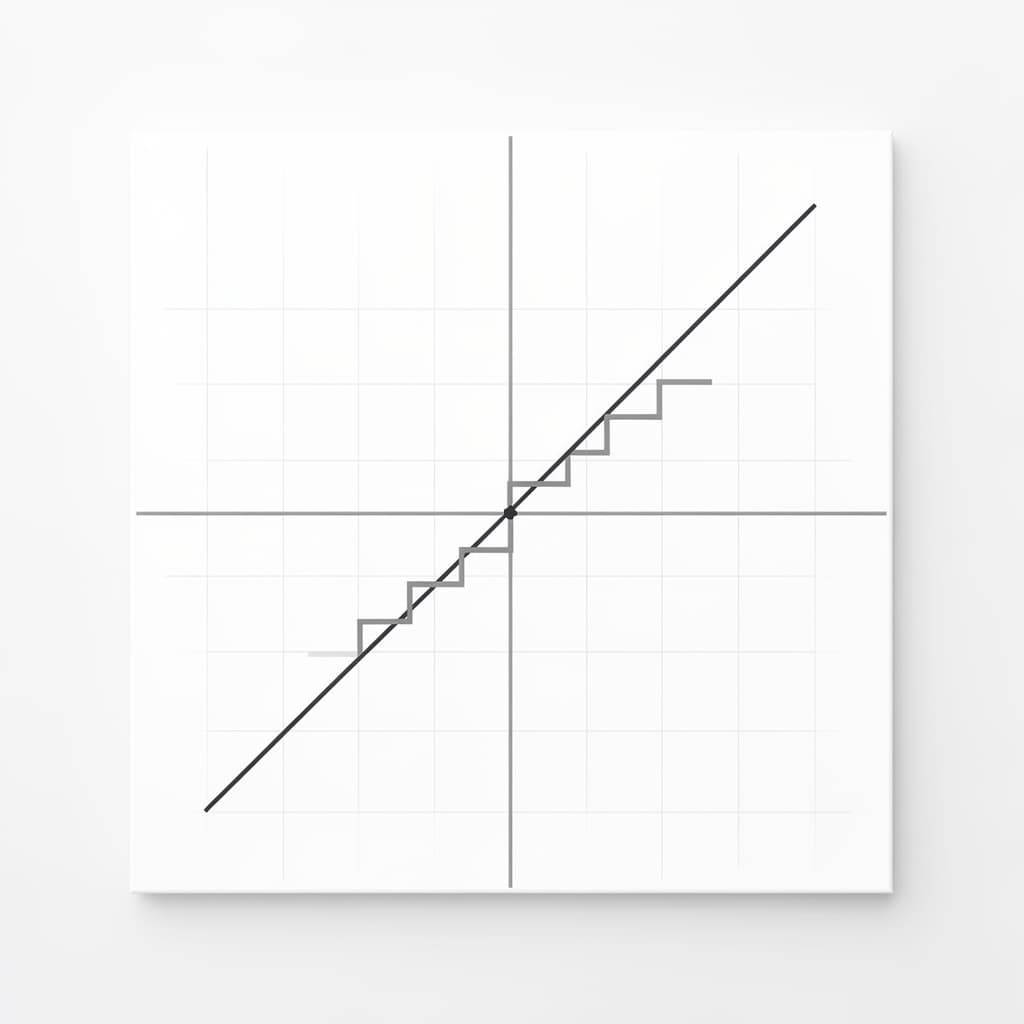
Once the y-intercept is plotted, the slope $m$ acts as a set of navigational instructions to find the next point. If the slope is written as a fraction, such as $3/4$, you "rise" three units up and "run" four units to the right from your starting point. If the slope is an integer like $-2$, you treat it as $-2/1$, meaning you move two units down and one unit to the right. Repeating this pattern allows you to generate an infinite number of points that all fall along the same straight path. This stair-step method of movement ensures that the line maintains a perfectly consistent angle across the graph.

Connecting Points to Reveal the Linear Pathway

The final step in the graphing process is to draw a straight line through the points you have plotted, extending it to the edges of the grid. It is standard practice to add arrows to both ends of the line to indicate that the linear relationship continues infinitely in both directions. This visual line represents every possible solution to the equation, showing that for every fractional $x$ value, there is a corresponding $y$ value. By connecting the points, you transform an abstract algebraic expression into a concrete geometric object. This visualization is essential for identifying where different lines might intersect or how they relate to the axes.

Algebraic Steps to Find the Equation of a Line

Deriving Formulas from Two Known Coordinates

A common challenge in algebra is to find the equation of a line when you are given only two sets of coordinates. The first step in this process is always to calculate the slope $m$ using the rise-over-run formula mentioned previously. Once the slope is determined, you can substitute the value of $m$ and the coordinates of one of the points into the $y = mx + b$ template. This leaves $b$ as the only unknown variable, which can then be isolated and solved for using basic arithmetic. For example, if you have a slope of 3 and the point $(1, 5)$, you set up the equation $5 = 3(1) + b$, which reveals that $b = 2$.

Utilizing the Point-Slope Method for Conversion

While $y = mx + b$ is the most popular form, the point-slope form is often used as an intermediate tool during derivation. The point-slope formula is written as $$y - y_1 = m(x - x_1)$$, where $m$ is the slope and $(x_1, y_1)$ is a known point. This version of the equation is particularly useful because it requires no initial solving for $b$; you simply plug in the numbers and then use distributive property to simplify. After distributing the slope and moving the $y_1$ term to the other side, the equation naturally transforms into the slope-intercept form. This two-step conversion process is the most reliable way to handle complex coordinates or fractional slopes.

Identifying Constants in Raw Numerical Data

In many scientific and statistical contexts, finding the equation of a line involves looking at a table of data rather than a pre-drawn graph. To identify the slope-intercept components, one must look for the "initial value," which is the $y$-value when $x$ is zero; this is your $b$. If the table does not include a zero for $x$, you must determine the rate at which $y$ changes for every one-unit increase in $x$ to find $m$. Once $m$ is known, you can work backward to find what $y$ would be at the zero-point. This analytical approach treats the slope-intercept form as a tool for discovering the underlying rules that govern a set of observations.

Illustrative Slope Intercept Form Examples

Walking Through a Basic Integer Coefficient Problem

To clarify the application of the formula, let us examine one of the most straightforward slope intercept form examples: $$y = 2x + 1$$. In this scenario, the slope $m$ is 2, and the y-intercept $b$ is 1. To graph this, we start by placing a point at $(0, 1)$ on the y-axis. Using the slope of 2 (which is $2/1$), we move up two units and right one unit to find the next point at $(1, 3)$. Connecting these points creates a line that climbs steadily, showing that for every step forward we take, the height of the line doubles that progress plus the starting offset of one.

Consider the calculation table for this specific equation to see the linear progression clearly:

Input (x)	Equation Calculation (2x + 1)	Output (y)
-1	2(-1) + 1	-1
0	2(0) + 1	1
1	2(1) + 1	3
2	2(2) + 1	5

Solving Equations with Fractional Slopes

Equations with fractional slopes, such as $y = \frac{1}{2}x - 3$, often intimidate students, but they follow the exact same logic. Here, the slope is $1/2$, which tells us that for every two units we move to the right (the run), the line only rises by one unit (the rise). The y-intercept is $-3$, meaning the line starts three units below the origin at $(0, -3)$. Fractional slopes result in "shallower" lines that do not climb or descend as aggressively as those with whole-number slopes. Mastering these fractions is key to understanding how to model subtle changes where the output grows more slowly than the input.

Addressing Negative Intercepts in Cartesian Space

Negative intercepts are a frequent occurrence and simply mean that the relationship starts in the negative territory of the vertical axis. For example, in the equation $y = -3x - 5$, the line crosses the y-axis at $-5$. Because the slope is $-3$, the line will then descend three units for every one unit it moves to the right. This results in a line that starts low and continues to plummet deeper into the negative quadrants of the graph. It is important to treat the negative sign as part of the constant $b$, ensuring that the "starting point" is correctly identified as a negative coordinate rather than a subtraction from a positive intercept.

Converting Standard Form to Slope-Intercept

The Process of Isolating the Y Variable

In many algebraic textbooks, equations are initially presented in Standard Form, written as $Ax + By = C$. While this form is useful for finding intercepts, it does not reveal the slope or the y-intercept as clearly as the slope-intercept form does. To convert it, the primary goal is to isolate $y$ on one side of the equal sign through a series of algebraic manipulations. This usually involves subtracting the $Ax$ term from both sides and then dividing the entire equation by the coefficient $B$. This process effectively "unpacks" the equation, reorganizing the constants into the recognizable $m$ and $b$ parameters.

"The transformation of an equation from standard form to slope-intercept form is essentially the process of solving for the dependent variable to reveal the rate of change."

Simplifying Expressions for Visual Clarity

Once $y$ is isolated, the resulting expression may contain fractions that need simplification to be useful for graphing. For instance, if you have $4y = -2x + 8$, dividing by 4 yields $y = -\frac{2}{4}x + \frac{8}{4}$, which simplifies to $y = -\frac{1}{2}x + 2$. Maintaining the slope as a simplified fraction is vital because it makes the "rise over run" instructions much easier to follow on a grid. Similarly, reducing the y-intercept to its simplest integer or decimal form allows for precise plotting on the axis. Clarity in notation leads to accuracy in visualization, which is why simplification is a non-negotiable step in the conversion process.

Common Algebraic Pitfalls During Transformation

The most frequent errors during conversion involve sign changes and division of multiple terms. When subtracting $Ax$ from both sides, students often forget to keep the negative sign attached to the $x$ term on the right side. Furthermore, when dividing by $B$ to isolate $y$, it is essential to divide every single term on the other side of the equation, not just the first one. If an equation is $2x - 3y = 9$, the division by $-3$ must be applied to both $2x$ and $9$, resulting in $y = \frac{2}{3}x - 3$. Attention to these small details prevents the entire line from being shifted or tilted incorrectly on the graph.

Applications in Coordinate Geometry

Interpreting Slopes as Constant Rates of Change

Beyond the classroom, the slope $m$ in the slope intercept form is almost always representative of a constant rate of change. In physics, the slope of a position-time graph represents velocity; in economics, the slope of a total cost graph represents marginal cost. Because the slope is constant in a linear equation, it implies that the relationship between the two variables never wavers. This predictability is what makes linear models so powerful for forecasting. If you know that a car travels at a constant speed, you can use the slope-intercept form to calculate exactly where it will be at any given point in time.

Analyzing Parallel and Perpendicular Line Relationships

The slope-intercept form is the most efficient tool for comparing the orientation of two different lines. Parallel lines are defined by having identical slopes ($m_1 = m_2$) but different y-intercepts, meaning they will travel in the same direction forever and never touch. Perpendicular lines, which intersect at perfect 90-degree angles, have slopes that are "negative reciprocals" of one another (for example, 2 and $-1/2$). By simply looking at the $m$ values of two equations, a mathematician can determine their geometric relationship without ever needing to draw them. This algebraic shorthand is fundamental to advanced fields like engineering and architectural design.

The Role of Linearity in Predictive Mathematics

Linearity is the foundation of predictive modeling, and the slope-intercept form is its most basic expression. Even in complex data sets that are not perfectly linear, researchers often use "linear regression" to find the line of best fit that most closely approximates the trend. This line, expressed as $y = mx + b$, allows scientists to make educated guesses about future data points based on historical rates of change. While the world is often non-linear and chaotic, the "elegant logic" of the straight line provides a necessary baseline for understanding growth, decay, and equilibrium in the physical and social sciences.

References

- Stewart, J., "Calculus: Early Transcendentals", Cengage Learning, 2020.
- Descartes, R., "The Geometry of René Descartes" (Translated by David Eugene Smith and Marcia L. Latham), Open Court Publishing Company, 1925.
- Sullivan, M., "Algebra & Trigonometry", Pearson, 2019.
- Axler, S., "Precalculus: A Prelude to Calculus", Wiley, 2016.
Recommended Readings
- Linear Algebra Done Right by Sheldon Axler — A deeper dive into the structures that govern linear equations and their applications in higher-dimensional spaces.
- The Joy of x: A Guided Tour of Math, from One to Infinity by Steven Strogatz — An accessible exploration of mathematical concepts, including how linear relationships define our everyday world.
- Coordinate Geometry by S.L. Loney — A classic foundational text for anyone looking to master the rigorous proofs and geometric origins of the Cartesian plane.