The Elegant Geometry of PID Control

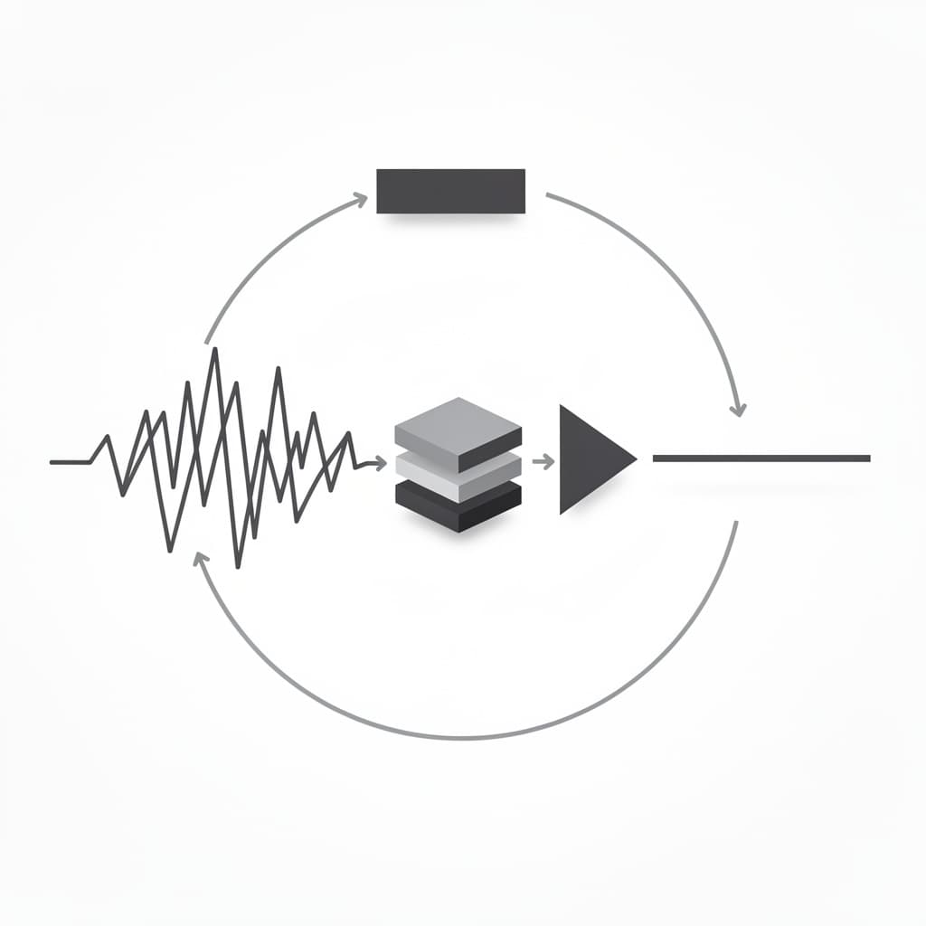
In the domain of automation and industrial engineering, few concepts possess the enduring utility and mathematical elegance of the Proportional-Integral-Derivative (PID) controller. At its core, understanding how pid controller works requires a shift from viewing machines as simple "on-off" devices to seeing them as dynamic entities capable of self-correction through mathematical feedback. Whether it is maintaining the precise altitude of a multi-million-dollar drone, regulating the temperature of a chemical reactor, or ensuring the smooth cruise control of a modern electric vehicle, the PID algorithm serves as the silent intelligence mediating between desired goals and physical reality. By continuously calculating the difference between a target setpoint and a measured process variable, the controller applies a correction that is simultaneously informed by the present, the past, and the predicted future.

Defining the Feedback Mechanism

Anatomy of a Closed-Loop Control System

To understand the functional logic of a PID controller, one must first visualize the architecture of a closed-loop control system. Unlike an open-loop system—such as a common toaster that runs for a fixed duration regardless of the bread's actual brownness—a closed-loop system relies on constant observation. The system consists of four primary components: the process (the machine being controlled), the sensor (which measures the current state), the controller (the brain), and the actuator (the device that exerts influence, like a heater or motor). The sensor provides the "feedback" that allows the controller to adjust its output dynamically, creating a continuous loop of measurement and correction that accounts for external disturbances. This cycle ensures that the system remains responsive to environmental changes, such as a sudden drop in ambient temperature or a change in mechanical load.

The elegance of this system lies in its autonomy; it does not require a human operator to constantly adjust a dial. Instead, the controller receives a Setpoint (SP), which represents the desired value, and compares it against the Process Variable (PV), which is the current value reported by the sensor. The difference between these two values is known as the error signal. A high-quality closed-loop system is characterized by its ability to reach the setpoint quickly, minimize overshoot (going past the target), and maintain stability over time. By closing the loop, engineers transform unpredictable physical processes into precise, repeatable operations that form the backbone of modern manufacturing and robotics.

The Fundamental Error Equation

The mathematical heart of any control logic is the calculation of error, denoted as $e(t)$. At any given moment in time $t$, the error is defined as the subtraction of the current measurement from the target goal. The formula is expressed simply as: $$e(t)=SP-PV(t)$$ This value is the raw data that the PID algorithm processes to determine its next move. If the error is zero, the system is exactly where it needs to be, and the controller ideally maintains its current state. However, if the error is positive, the system is below the target; if negative, it has exceeded the target. This sign and magnitude of the error dictate the direction and intensity of the controller's response.

The error signal is rarely a static number because physical systems are constantly subject to disturbances. Imagine a heating element in a room; the opening of a window introduces a disturbance that causes the PV (room temperature) to drop, thereby increasing the error $e(t)$. The PID controller’s job is to look at this error through three different mathematical lenses to decide how much power to send to the heater. By quantifying the gap between "what is" and "what should be," the error equation provides the foundational logic for the proportional, integral, and derivative calculations that follow. Without this clear mathematical definition of failure (the error), the system would have no objective basis for improvement.

What is a PID Controller

Broadly speaking, what is a pid controller can be answered as a control loop mechanism that uses feedback to maintain a process at a desired state. It is a mathematical formula implemented in software or hardware that combines three distinct modes of correction. The "P" (Proportional) accounts for the current error, the "I" (Integral) accounts for the accumulation of past errors, and the "D" (Derivative) accounts for the predicted future error based on the current rate of change. By summing these three components, the controller produces a single output signal, often called the Control Variable (CV) or Manipulated Variable (MV), which is sent to the actuator.

The history of the PID controller dates back to the early 20th century, notably popularized by Nicolas Minorsky in 1922 for the automatic steering of US Navy ships. Minorsky observed that human helmsmen corrected the ship's course not just based on the current deviation, but also by how long they had been off course and how fast the ship was swinging. Today, PID controllers are no longer mechanical governors but are primarily found in Programmable Logic Controllers (PLCs) and microcontrollers. Their ubiquity stems from their versatility; they can be applied to almost any linear system without requiring a complex mathematical model of the process itself. This "black box" capability makes them the gold standard for engineers across various industries.

The Proportional Action of Direct Response

Scaling the Error with Gain

The Proportional component is the most intuitive part of the PID algorithm, often described as the "present" response. It produces an output that is directly proportional to the current error value. If the error is large, the correction is large; if the error is small, the correction is small. This is achieved by multiplying the error $e(t)$ by a constant factor known as the Proportional Gain ($K_p$). The mathematical expression for the proportional term is: $$P_{out}=K_{p}e(t)$$ A higher $K_p$ value means the controller will react more aggressively to any deviation from the setpoint, essentially making the system more sensitive and faster to respond.

In a real-world scenario, such as a driver steering a car, the proportional action is equivalent to how far the driver turns the steering wheel in response to being off-center. If the car is slightly to the left, the driver turns the wheel slightly to the right. If the car is veering sharply off the road, the driver applies a much larger turn. However, if the gain is set too high, the system can become unstable. The controller may overreact to a small error, causing the system to overshoot the setpoint and then over-correct in the opposite direction, leading to a state of perpetual oscillation. Tuning the proportional gain is therefore a delicate balance between achieving a rapid response and maintaining a smooth, controlled approach to the target.

Limitations and the Steady State Offset

While proportional control is powerful, it suffers from a fundamental mathematical limitation known as steady-state offset or "droop." Because the proportional output is calculated by multiplying the error, the output effectively becomes zero when the error is zero. In many physical systems, a certain amount of constant output is required to maintain the setpoint. For example, if you are trying to hold a drone at a specific altitude, the motors must always be spinning to fight gravity. If the proportional controller successfully reaches the target altitude, the error becomes zero, the output drops to zero, and the drone falls. As the drone falls, the error increases again, and the controller provides power, eventually finding an equilibrium point below the target altitude where the proportional output perfectly balances the force of gravity.

This gap between the equilibrium point and the actual setpoint is the steady-state error. Increasing the gain $K_p$ can reduce the size of this offset, as it allows a smaller error to generate a larger output, but it can never eliminate it entirely without causing instability. This is why a purely proportional controller is rarely used in applications requiring high precision. To solve the problem of the persistent offset, we must look beyond the "present" error and consider the history of the system's performance. This necessity leads directly to the introduction of the Integral term, which provides the memory required to close the remaining gap.

Eliminating Residual Error via Integration

Accumulating the History of Deviation

The Integral component of the PID controller is designed to eliminate the steady-state offset by looking at the "past" behavior of the error. Instead of just looking at how big the error is right now, the integral term sums (integrates) the error over time. Even if the error is very small, if it persists for a long duration, the integral term will grow larger and larger, eventually forcing the controller to increase its output until the error is driven to zero. The mathematical representation involves the Integral Gain ($K_i$) and the integral of the error over time: $$I_{out}=K_i{\int }_0^{t}e(\tau )d\tau$$ In practical terms, the integral action "remembers" that the system has been below the setpoint for a while and adds more "effort" to push it toward the target.

Consider a water tank where the goal is to maintain a specific water level. If a small leak exists, a proportional-only controller might settle at a level just below the target because the small error generates just enough inflow to match the leak. The integral term, however, sees this persistent small gap and begins to accumulate. It slowly "ramps up" the inflow valve's position until the water level exactly reaches the setpoint. Once the error is zero, the integral term stops growing, but it retains the value it has already accumulated. This allows the controller to maintain a non-zero output (the inflow needed to offset the leak) even when the error is zero, successfully solving the limitation of the proportional-only approach.

Managing the Risk of Integral Windup

While the integral action is essential for accuracy, it introduces a specific engineering challenge known as Integral Windup. This occurs when a large change in the setpoint happens, or the actuator reaches its physical limit (saturation). For example, if a heater is already at 100 percent power but the temperature is still below the target, the error remains positive. The integral term will continue to accumulate and grow to a massive value because the error isn't going away. Once the temperature finally reaches the setpoint, the integral term is so large that it keeps the heater at 100 percent power for a long time, causing a massive and potentially dangerous overshoot before the "wound up" integral can be discharged.

To prevent this, modern PID implementations include "anti-windup" logic. This can involve clamping the integral term to a maximum value or pausing the integration whenever the actuator is saturated. By preventing the integral term from growing beyond the physical capabilities of the system, engineers ensure that the controller remains responsive and can quickly recover once the error begins to decrease. Properly managing the integral action is the difference between a system that settles perfectly at its target and one that oscillates wildly or damages itself through excessive correction. This highlights the importance of not just mathematical theory, but practical safeguards in how pid controller works in industrial environments.

Anticipating Change with Derivative Control

Predicting Future Error Trends

The Derivative component provides the "future" or "predictive" aspect of the PID controller. It calculates the rate of change of the error signal over time. If the error is decreasing rapidly, the derivative term produces a negative value that "brakes" the controller's output, preventing the system from overshooting the setpoint. Conversely, if the error is suddenly increasing, the derivative term adds an extra boost to stop the deviation as quickly as possible. The formula for the derivative term involves the Derivative Gain ($K_d$) and the slope of the error: $$D_{out}=K_d\frac{de(t)}{dt}$$ This action acts as a damper, providing stability and reducing the oscillations that can be caused by the proportional and integral terms.

A classic analogy for derivative control is a driver approaching a red light. A proportional-only driver would wait until they are very close to the light to brake hard. A derivative-aware driver notices the rate at which they are approaching the light and begins to apply the brakes early and smoothly. This anticipatory behavior allows for much higher proportional gains to be used without the risk of instability. By "sensing" the speed of the error's movement, the derivative term allows the system to react not just to where it is, but to where it is heading, creating a much more sophisticated and human-like response to changes in the environment.

Sensitivity to Signal Noise and Fluctuations

Despite its benefits in providing stability and speed, the derivative term is the most problematic to implement in real-world systems because of its extreme sensitivity to signal noise. In any electronic system, sensors produce slight, high-frequency fluctuations in their readings due to electromagnetic interference or mechanical vibrations. Because the derivative calculates the rate of change, even a tiny, near-instantaneous jump in sensor data can result in a massive derivative value (since the change over a very small time is mathematically a large slope). This can cause the controller's output to jitter or "chatter," which puts unnecessary wear on mechanical actuators like valves and motors.

To mitigate this, derivative action is rarely applied to the raw error signal in industrial applications. Instead, it is often applied to a filtered version of the Process Variable. Engineers typically use a low-pass filter to smooth out high-frequency noise before it reaches the derivative calculation, ensuring that the controller only reacts to genuine trends in the data rather than random fluctuations. In some systems where noise is particularly high or where the process moves very slowly (like large thermal masses), the derivative term is set to zero, resulting in a PI controller. Understanding when to use or omit the "D" term is a critical skill in pid tuning guide methodologies, as the wrong application can lead to more harm than good.

The Proportional Integral Derivative Synergy

Combining the Three Mathematical Terms

The true power of the proportional integral derivative controller emerges when the three terms are combined into a single, unified equation. This synergy allows the controller to handle the present, past, and future of the system simultaneously. The ideal parallel form of the PID equation is: $$u(t)=K_{p}e(t)+K_i{\int }_0^{t}e(\tau )d\tau +K_d\frac{de(t)}{dt}$$ In this equation, $u(t)$ is the final control signal sent to the actuator. Each term provides a unique contribution: the Proportional term provides the bulk of the "muscle" to move the system, the Integral term provides the "persistence" to ensure total accuracy, and the Derivative term provides the "finesse" to prevent overshooting and maintain stability.

In many commercial controllers, the equation is written in a slightly different "standard" form, where the gains are expressed as a single controller gain $K_c$ and two time constants: Integral Time ($T_i$) and Derivative Time ($T_d$). This version looks like this: $$u(t)=K_c\left(e(t)+\frac{1}{T_i}{\int }_0^{t}e(\tau )d\tau +T_d\frac{de(t)}{dt}\right)$$ Regardless of the form, the fundamental logic remains the same. The controller is constantly weighing these three influences, balancing the need for speed against the need for stability. When these three mathematical forces are correctly balanced, the result is a system that responds to setpoint changes with surgical precision, settling onto the new target with minimal delay and no residual error.

Balancing Speed and Stability

Finding the perfect balance between the P, I, and D components is the central challenge of control engineering. A system that is too fast (high $K_p$) will oscillate and potentially become unstable, while a system that is too stable (high $K_d$ or low $K_p$) will be sluggish and slow to respond to disturbances. The interaction between the terms is complex; for instance, increasing the Integral gain ($K_i$) helps eliminate error faster, but it also reduces the stability of the system, often requiring an increase in the Derivative gain ($K_d$) to compensate. This intricate dance of variables is what makes PID control an "elegant geometry" of logic.

To visualize this balance, engineers often use a step response graph, which shows how the system reacts to a sudden change in the setpoint. An underdamped system will reach the target quickly but ring like a bell, overshooting the target several times. An overdamped system will approach the target without any overshoot but will take a very long time to get there. The "Goldilocks" zone is known as a critically damped response, where the system reaches the target as fast as possible without overshooting. Achieving this state requires precise tuning, which is both a science of mathematics and an art of observation, involving careful adjustment of the three gain parameters to suit the specific physics of the machine being controlled.

A Comprehensive PID Tuning Guide

The Ziegler-Nichols Heuristic Approach

For decades, the Ziegler-Nichols method has been the most famous heuristic for pid tuning guide procedures. Developed in the 1940s, this method provides a structured way to find initial PID values without needing a mathematical model of the system. The process begins by setting the Integral and Derivative gains to zero. The Proportional gain ($K_p$) is then slowly increased until the system reaches a state of "ultimate oscillation," where it continuously bounces back and forth at a constant amplitude. This specific gain is called the Ultimate Gain ($K_u$), and the period of these oscillations is called the Ultimate Period ($P_u$).

Once $K_u$ and $P_u$ are measured, the PID parameters are calculated using a standardized table of coefficients. While these values often require further refinement, they provide a mathematically sound starting point that is much safer and more efficient than blind guessing. The following table summarizes the classic Ziegler-Nichols tuning rules:

Control Type	$K_p$	$T_i$ ($1/K_i$)	$T_d$ ($K_d$)
Proportional (P)	$0.50K_u$	-	-
PI Control	$0.45K_u$	$P_u/1.2$	-
PID Control	$0.60K_u$	$P_u/2$	$P_u/8$

Manual Trial and Error Methodologies

While formal methods like Ziegler-Nichols are useful, many engineers rely on a manual tuning approach, which allows for more intuitive control over the system's "feel." The general strategy is to start with a P-only controller to establish a basic response. Once the system is responding reasonably quickly (even with an offset), the Integral gain is slowly increased to pull the Process Variable toward the Setpoint and eliminate the offset. If the introduction of the Integral term causes the system to start oscillating or "hunting" for the target, the Proportional gain is slightly reduced, or a small amount of Derivative gain is added to dampen the movement.

A helpful tip in manual tuning is the "Rule of Halves and Doubles." If the system is clearly unstable, cut the gain in half; if it is clearly too slow, double it. This logarithmic approach helps you narrow in on the correct order of magnitude much faster than linear adjustments. It is also important to test the tuning under various conditions—for example, a heater might behave differently when the room is cold versus when it is already warm. High-quality tuning ensures that the PID parameters are robust enough to handle the entire operating range of the machine, providing consistent performance regardless of external variables or aging components.

Real-World PID Control Examples

Thermal Regulation in Industrial Furnaces

One of the most common pid control examples is the regulation of temperature in industrial furnaces or chemical reactors. These systems are characterized by large "dead times" and "thermal inertia," meaning that when you turn on a heater, it takes a significant amount of time before the sensor detects a change in temperature. In these cases, a simple on-off controller would cause massive temperature swings, potentially ruining chemical batches or damaging materials. A PID controller, however, can be tuned to account for this lag. The Proportional term handles the bulk of the heating, while the Integral term ensures that the furnace stays exactly at the target temperature despite heat loss through the furnace walls.

In thermal systems, the Derivative term is often used sparingly because temperature changes occur relatively slowly, and noise in thermocouple sensors can be significant. However, a small amount of Derivative action can be vital when a new, cold load is placed into the furnace. The "D" term senses the sudden drop in temperature and the rapid rate of change, prompting the controller to surge the power immediately before the Integral term even has a chance to accumulate. This prevents the furnace from staying cold for too long, maintaining the tight tolerances required in semiconductor manufacturing or aerospace metallurgy, where even a few degrees of deviation can lead to catastrophic material failure.

Precision Stability in Modern Avionics

In the high-stakes world of avionics, PID controllers are used to maintain the stability of aircraft and drones. A quadcopter, for instance, is inherently unstable; without a computer constantly adjusting the speed of its four motors, it would flip over and crash in milliseconds. Here, the PID loop runs at very high frequencies, often 400 times per second (400Hz) or more. The "Process Variable" is the drone's current angle (measured by a gyroscope), and the "Setpoint" is the angle commanded by the pilot's joystick. The PID controller must respond almost instantly to wind gusts or rapid maneuvers to keep the drone level.

In this application, the Derivative term is arguably the most important. Because air is a low-friction medium, a drone can easily start to oscillate if it moves too quickly. The Derivative action acts as "electronic molasses," providing a counter-force that grows stronger as the drone rotates faster, effectively smoothing out the flight and making the craft feel "locked in." This is why racing drone pilots spend hours fine-tuning their "D-term" to achieve the perfect balance between snappy response and buttery-smooth video footage. This illustrates how pid controller works to tame chaotic physical forces into predictable, high-performance motion.

Implementation in Digital Architecture

Discrete Time Domain Conversion

While the classic PID theory is based on continuous calculus (integrals and derivatives), modern controllers operate in the discrete time domain. Microprocessors cannot "integrate" a continuous signal; instead, they sample the sensor at specific intervals ($T_s$) and perform calculations on those samples. The integral is approximated as a sum of error rectangles (Riemann sum), and the derivative is approximated as the difference between the current error and the previous error divided by the sample time. The transition from the continuous formula to digital code is essential for implementation in embedded systems and PLCs.

The discrete-time version of the PID equation for a single time step $n$ is often written as: $$u[n]=K_{p}e[n]+K_i\sum _{i=0}^{n}e[i]\Delta t+K_d\frac{e[n]-e[n-1]}{\Delta t}$$ This version is easy to program into a computer. To make the code more efficient and avoid the "integral windup" mentioned earlier, engineers often use the "velocity form" or "incremental form" of the algorithm, which calculates how much the output should change from the last step, rather than calculating the total output from scratch. This makes it easier to handle actuator limits and provides a smoother transition when switching the controller from manual to automatic mode.

Microcontroller Logic and Sampling Rates

The performance of a digital PID controller is heavily dependent on its sampling rate. If the controller samples the sensor too slowly, it becomes "blind" to what is happening between samples, which can lead to instability—much like trying to drive a car while only opening your eyes for half a second every five seconds. A general rule of thumb is that the sampling rate should be at least 10 to 20 times faster than the "time constant" or the fastest response of the system. In high-speed robotics, this might mean a sampling interval of 1 millisecond, whereas in a slow-moving water tank, a sampling interval of 1 second might be perfectly adequate.

Implementing a PID controller in code also requires careful attention to data types and precision. Using floating-point math provides the best accuracy but can be slow on cheap microcontrollers. Many industrial systems use "fixed-point" math to speed up calculations. Below is a simplified example of how pid controller works when translated into a pseudo-code implementation that can be adapted for platforms like Arduino or C++ based PLCs:

// Standard PID calculation loop
double computePID(double target, double current) {
    static double integral = 0;
    static double lastError = 0;
    
    double error = target - current;
    double derivative = (error - lastError) / dt;
    integral += error * dt;
    
    // Apply gains and sum the terms
    double output = (Kp * error) + (Ki * integral) + (Kd * derivative);
    
    lastError = error;
    return output;
}

This simple logic, repeated thousands of times per second, is what enables the high-precision world we live in. From the temperature of your coffee machine to the stability of the International Space Station, the PID controller remains the most successful and widely used algorithm in the history of control theory. Its ability to manage the complexities of the physical world using three simple mathematical concepts—proportionality, integration, and differentiation—is a testament to the power of elegant engineering.

References

- Åström, K. J., & Hägglund, T., "Advanced PID Control", ISA (International Society of Automation), 2006.
- Ogata, K., "Modern Control Engineering", Prentice Hall, 2010.
- Minorsky, N., "Directional Stability of Automatically Steered Bodies", Journal of the American Society for Naval Engineers, 1922.
- Ziegler, J. G., & Nichols, N. B., "Optimum Settings for Automatic Controllers", Transactions of the ASME, 1942.
- Knuth, D. E., "The Art of Computer Programming, Vol. 2: Seminumerical Algorithms", Addison-Wesley, 1997.
Recommended Readings
- Feedback Systems: An Introduction for Scientists and Engineers by Karl Johan Åström and Richard M. Murray — An incredibly deep but accessible dive into the mathematics of feedback and stability that underpins all control theory.
- PID Controllers: Theory, Design, and Tuning by Karl J. Åström and Tore Hägglund — Considered the "bible" of PID control, this book offers practical insights for industrial applications and rigorous mathematical proofs.
- The Control Handbook by William S. Levine — A comprehensive reference that covers everything from the basics of PID to advanced non-linear and optimal control strategies.
- Designing Linear Control Systems with MATLAB by Katsuhiko Ogata — A practical guide for those who want to use simulation software to model and tune PID controllers in a virtual environment.
Turn this topic into a full course
Noesis builds the syllabus, notes and tests for you, and you study them with a tutor that knows your material.