The Computational Logic of Big O Notation

In the realm of computer science, the efficiency of an algorithm is not measured by the seconds it takes to execute on a specific machine, but by how its resource requirements scale as the input grows. This brings us to the fundamental question: what is big o notation? At its core, Big O notation is a mathematical formalization used to describe the upper bound of an algorithm's running time or memory usage in the worst-case scenario. By stripping away hardware dependencies, compiler optimizations, and constant factors, Big O allows engineers to compare the inherent logic of different approaches. It serves as a lingua franca for developers, ensuring that when we discuss performance, we are focused on the asymptotic behavior of the code rather than transient environmental variables.

Foundations of Asymptotic Analysis

Asymptotic analysis provides a framework for evaluating the performance of algorithms by focusing on their behavior as the input size, denoted as $n$, approaches infinity. In this context, the specific execution time on a high-end server versus a legacy laptop becomes irrelevant because we are interested in the growth rate of the function. For instance, an algorithm that processes a list of ten items may run instantly regardless of its design, but the difference between a linear and a quadratic approach becomes catastrophic when that list grows to ten million items. Asymptotic analysis allows us to categorize functions into classes based on how quickly their requirements accelerate, providing a high-level view of scalability that transcends specific implementation details.

The mathematical abstraction of Big O notation relies on the concept of the upper bound limit. Formally, a function $f(n)$ is said to be $O(g(n))$ if there exist positive constants $c$ and $n_0$ such that $0 \le f(n) \le c \cdot g(n)$ for all $n \ge n_0$. This means that beyond a certain "break-even" point, the actual running time of the algorithm will never exceed the growth of $g(n)$ multiplied by some constant factor. This abstraction is powerful because it simplifies complex polynomials into their most significant terms. For example, if an algorithm has a step count represented by $3n^2 + 10n + 5$, we discard the lower-order terms ($10n + 5$) and the constant coefficient ($3$), simplifying the complexity to $O(n^2)$.

Understanding growth rates requires a shift in perspective from absolute numbers to relative proportions. When we ask what is big o notation, we are really asking how the workload changes when the input doubles. In a linear system, doubling the input doubles the work; in a quadratic system, doubling the input quadruples the work. This predictive power is essential for software architects who must decide whether a proposed solution will remain viable as a platform's user base expands. By prioritizing the highest-order term, Big O notation highlights the primary bottleneck of an algorithm, allowing developers to focus their optimization efforts where they will have the most significant long-term impact.

Decoding Time Complexity Explained

Time complexity is often the most critical metric in algorithm analysis, as it directly impacts user experience and system throughput. The simplest complexity class is $O(1)$, or constant time, where the execution time remains the same regardless of the input size. An example of this is accessing an element in an array by its index; the computer performs a single memory address calculation, which takes the same amount of effort whether the array has five elements or five billion. While $O(1)$ is the gold standard of efficiency, it is rarely achievable for complex data processing tasks that require inspecting every piece of information provided.

When an algorithm must touch every input element exactly once, it falls into the category of $O(n)$, or linear time. This is common in simple search operations or totalizing a list of numbers, where the time taken scales in direct proportion to the size of the data set. Beyond linear time, we encounter $O(\log n)$, or logarithmic complexity, which is the hallmark of efficient searching in sorted structures like binary trees. Logarithmic efficiency is highly desirable because the number of operations grows very slowly; for example, doubling the input size only adds a single additional step to the process, making it incredibly effective for massive datasets.

On the opposite end of the spectrum lie polynomial and exponential growth rates, which represent significant challenges for scalability. Quadratic complexity, $O(n^2)$, typically occurs when an algorithm involves nested loops, where for every element in the input, we iterate through the input again. Even more dangerous is $O(2^n)$, or exponential time, where each new element in the input doubles the total number of operations. Such algorithms quickly become computationally infeasible even for relatively small values of $n$, often appearing in "brute-force" solutions to combinatorial problems. Understanding these distinctions is the first step in time complexity explained through the lens of mathematical logic.

Practical Big O Notation Examples

To ground these theoretical concepts, let us examine big o notation examples in standard programming patterns. Consider a basic function that checks for the existence of duplicates in a list using a nested loop. For each element $i$, the code iterates through every other element $j$ to check for equality. Because both the outer and inner loops run $n$ times, the total number of comparisons is $n \cdot n$, resulting in $O(n^2)$ complexity. If the list contains 1,000 items, the code performs one million comparisons, but if the list grows to 100,000 items, the number of comparisons balloons to ten billion, potentially freezing the application.

# Example of O(n^2) - Quadratic Complexity
def find_duplicates(items):
    for i in range(len(items)):
        for j in range(i + 1, len(items)):
            if items[i] == items[j]:
                return True
    return False

Contrast this with a "divide and conquer" strategy, such as the Merge Sort algorithm. Merge Sort recursively splits an array in half until it reaches single-element sub-arrays, then merges them back together in sorted order. The splitting phase creates a tree structure with $\log n$ levels, and at each level, $n$ work is done to merge the sub-arrays. This results in a total complexity of $O(n \log n)$, which is significantly more efficient than $O(n^2)$ for large inputs. In big o notation examples, $O(n \log n)$ is often the target for general-purpose sorting and complex data manipulation because it balances structural overhead with processing speed.

Recursive branching provides another fascinating look at complexity, particularly in the calculation of Fibonacci sequences. A naive recursive implementation of Fibonacci calls itself twice for every level of depth, creating a binary tree of function calls. The number of nodes in this tree grows at an exponential rate, leading to $O(2^n)$ complexity. This explains why calculating the 50th Fibonacci number using this method can take several minutes, while a linear approach using a simple loop ($O(n)$) or dynamic programming would finish in a fraction of a millisecond. These real-world examples illustrate that the choice of algorithm often matters more than the speed of the processor executing it.

The Space Complexity Guide

While time is a finite resource, so is memory, making a space complexity guide essential for robust software design. Space complexity measures the total amount of memory an algorithm requires relative to the input size. It is important to distinguish between auxiliary space—the extra space or temporary memory used by the algorithm—and the space occupied by the input itself. For example, an "in-place" sorting algorithm like QuickSort uses $O(\log n)$ auxiliary space for its recursive stack, whereas a non-in-place version might require $O(n)$ extra space to store copies of the sub-arrays. In memory-constrained environments like embedded systems or mobile devices, minimizing auxiliary space is often as critical as optimizing execution time.

Recursive algorithms introduce unique space challenges due to the call stack. Every time a function calls itself, a new "stack frame" is created in memory to store local variables and the return address. If a recursive function dives $n$ levels deep, it will consume $O(n)$ space on the stack even if it doesn't explicitly allocate any large data structures. This can lead to a "stack overflow" error if the recursion is too deep. Modern compilers sometimes optimize this via tail-call optimization, but in general, developers must be wary of how recursive depth impacts the memory footprint of their applications.

Buffer management and the choice of data structures also play a pivotal role in space complexity. Using a hash map to count the occurrences of characters in a string of length $n$ results in $O(k)$ space complexity, where $k$ is the size of the character set (e.g., 256 for extended ASCII). If $k$ is constant and small, this is effectively $O(1)$ space. However, if the algorithm creates a new list that grows with the input, the space complexity becomes $O(n)$. Balancing the trade-off between speed and memory—often called the space-time trade-off—is a core task of the software engineer, as using extra memory (like caches or memoization tables) can frequently reduce the time complexity of an operation.

Worst Case vs Best Case Analysis

In the mathematical study of algorithms, we must account for the fact that the same code can perform differently depending on the specific arrangement of the input data. This leads to the distinction of worst case vs best case analysis. The "Best Case," represented by Big Omega notation ($\Omega$), describes the minimum number of steps required under ideal conditions. For instance, in a linear search for a value in an array, the best case is finding the item at the very first index ($O(1)$). While interesting, best-case analysis is rarely used in isolation because it provides a misleadingly optimistic view of an algorithm's reliability.

Worst-case analysis, which is what Big O notation specifically identifies, focuses on the most pessimistic scenario. This is the most important metric for engineering because it allows us to provide guaranteed performance bounds. If we know an algorithm is $O(n^2)$, we can confidently state that it will never perform worse than that, regardless of how "messy" the input data is. There is also Average Case Analysis, which uses probability to determine the expected performance on a random input. While more representative of real-world usage, average-case analysis is mathematically complex and often depends on assumptions about the distribution of data that may not hold true in every environment.

A more nuanced approach is amortized analysis, which is used for operations that are expensive occasionally but inexpensive most of the time. A classic example is the dynamic array (like Python's list or Java's ArrayList). When the array is full and a new element is added, the system must allocate a larger block of memory and copy all existing elements, an $O(n)$ operation. However, because this happens so infrequently, the average cost over a long sequence of additions is actually $O(1)$. Amortized analysis prevents us from being overly discouraged by a single "slow" step, providing a fairer assessment of the algorithm's long-term performance in a dynamic system.

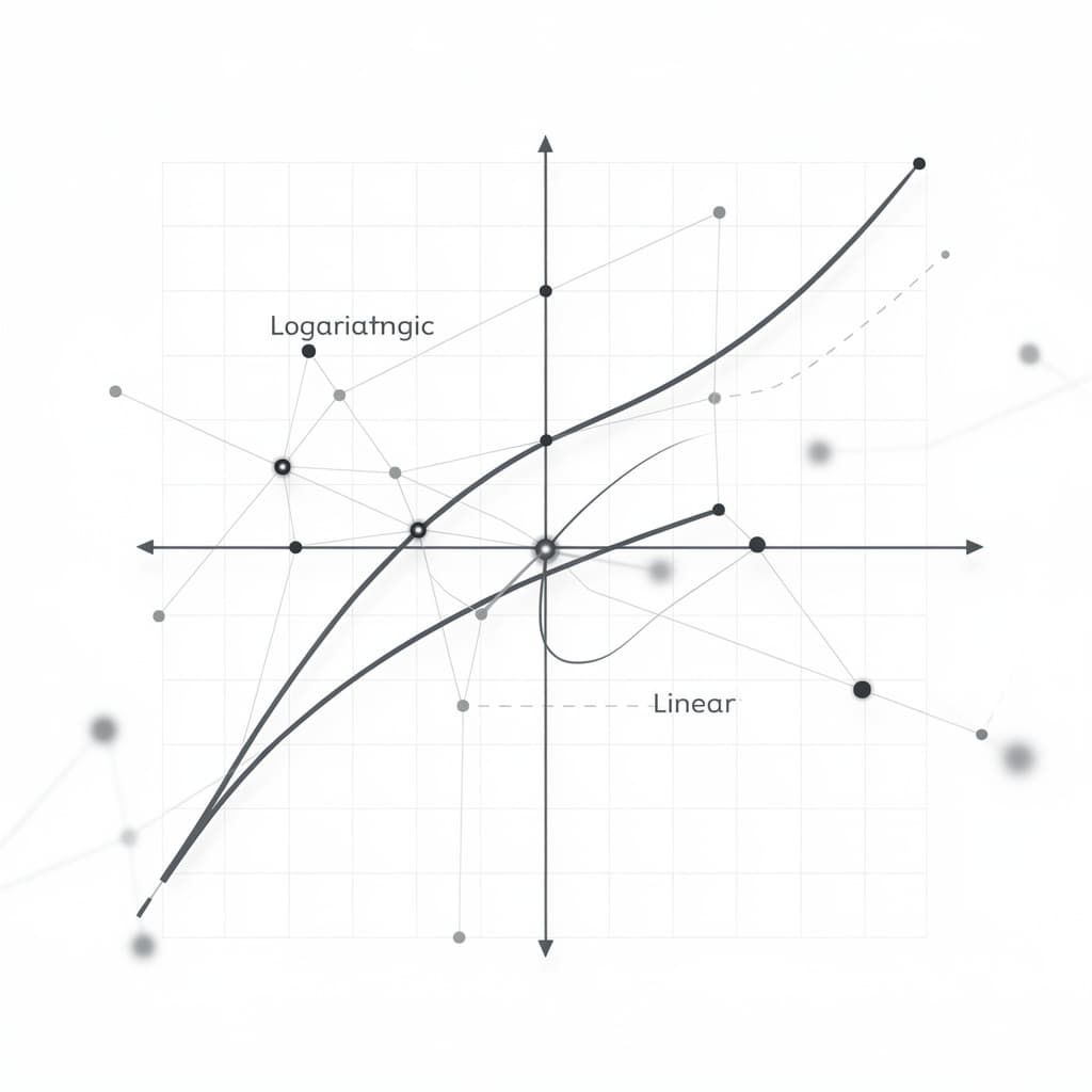
Visualizing the Algorithm Efficiency Chart

Visualizing the growth of different complexity classes on an algorithm efficiency chart is one of the most effective ways to build intuition. On such a chart, the $x$-axis represents the input size ($n$) and the $y$-axis represents the number of operations. At small values of $n$, the differences between $O(n)$, $O(n \log n)$, and $O(n^2)$ might be negligible. In fact, a "slower" algorithm might actually be faster for small datasets because it has a smaller constant factor (less overhead to start up). However, as $n$ increases, the curves begin to diverge sharply, and the "higher-order" algorithms eventually skyrocket toward the top of the chart.

The cross-over point is the specific input size where a theoretically more efficient algorithm finally becomes faster than a simpler one. For example, if Algorithm A is $100n$ and Algorithm B is $n^2$, Algorithm A is actually slower for any $n$ less than 100. This is why in practice, libraries for sorting often use a hybrid approach: they use a complex $O(n \log n)$ sort like Merge Sort for large arrays, but switch to a simple $O(n^2)$ Insertion Sort when the sub-arrays become small enough. Recognizing that Big O notation describes asymptotic behavior (at the limit) helps developers remember that for very small data, the simplicity of the implementation often trumps the theoretical complexity.

Complexity Class	Name	Impact of Doubling Input	Feasibility for Large $n$
$O(1)$	Constant	No change	Excellent
$O(\log n)$	Logarithmic	Negligible increase	Excellent
$O(n)$	Linear	Work doubles	Good
$O(n \log n)$	Linearithmic	Slightly more than double	Good
$O(n^2)$	Quadratic	Work quadruples	Poor
$O(2^n)$	Exponential	Work squares	Impossible

Finally, we must consider hardware constraints versus theoretical limits. While Big O focuses on the logic, physical reality involves CPU cache hits, branch prediction, and memory latency. An algorithm with $O(n)$ complexity that involves random memory access might actually perform worse than an $O(n \log n)$ algorithm that accesses memory sequentially due to the way modern processors handle data. Therefore, the efficiency chart should be viewed as a theoretical guide rather than an absolute law. It tells us what will happen as $n$ goes to infinity, but the "constant factors" hidden by Big O are what we optimize once the general complexity class is selected.

Higher-Level Complexity Classes

Beyond the standard complexities used in daily programming, computer scientists explore higher-level classes that define the limits of what is computable. The P vs NP problem is the most famous unsolved mystery in this field. "P" (Polynomial time) refers to problems that can be solved efficiently, while "NP" (Nondeterministic Polynomial time) refers to problems where a solution can be verified efficiently, even if it is hard to find. If a problem is "NP-Complete," it is considered intractable; as the input grows, no known algorithm can find a solution in a reasonable amount of time. This includes famous challenges like the Traveling Salesperson Problem or the Knapsack Problem.

In these high-complexity spaces, we encounter growth rates like $O(n!)$, or factorial time, and even double exponential growth. To put $O(n!)$ in perspective, if $n$ is only 20, the number of operations is approximately 2.4 quintillion. Because these problems cannot be solved perfectly for large inputs, computer scientists rely on heuristics and approximation algorithms. These are "good enough" solutions that provide a result close to the optimum in polynomial time. Understanding these boundaries prevents developers from wasting weeks trying to find a perfect, fast solution for a problem that is mathematically proven to be intractable.

The study of complexity also includes Space Complexity Classes like PSPACE, which contains problems that can be solved using a polynomial amount of memory, regardless of how much time they take. Interestingly, PSPACE is a broader category than P and NP, encompassing games like Chess or Go if played on an $n \times n$ board. These theoretical constructs may seem far removed from web development or data science, but they provide the essential map of the "computational landscape," helping us understand which problems are easy, which are hard, and which are effectively impossible for classical computers to solve.

Designing Scalable Software Architecture

In the world of system design, Big O notation is the primary tool for bottleneck identification. When a system slows down, it is rarely because every part of the code is slow; usually, one specific function or database query with a high complexity class is consuming the majority of the resources. By applying the logic of what is big o notation to entire architectural tiers, engineers can predict how their infrastructure will handle a ten-fold increase in traffic. If a microservice performs an $O(n^2)$ operation on a user's data every time they log in, the service will inevitably collapse as the user base grows, no matter how many servers are added to the cluster.

Scalable architecture involves making conscious trade-offs between memory and speed. For instance, using a Global Index or a Cache is an $O(1)$ lookup that requires $O(n)$ space. This is almost always a winning trade-off in web environments where latency is the primary concern. Furthermore, algorithmic refinement strategies often involve moving from a "naive" implementation to one that leverages more sophisticated data structures. Replacing a list with a Balanced Binary Search Tree or a Hash Table can transform an $O(n)$ lookup into $O(\log n)$ or $O(1)$, which is the difference between a system that feels sluggish and one that feels instantaneous.

Ultimately, designing for scale requires a deep respect for the "asymptotic wall." No amount of hardware can overcome the physics of an exponential algorithm once $n$ becomes sufficiently large. This makes the computational logic of Big O notation not just an academic exercise, but a mandatory skill for professional software development. By understanding growth rates, space-time trade-offs, and worst-case bounds, developers can write code that remains performant and reliable in the face of ever-increasing data demands. The mastery of these concepts ensures that the software of today can become the robust foundation for the innovations of tomorrow.

References

- Cormen, T. H., Leiserson, C. E., Rivest, R. L., & Stein, C., "Introduction to Algorithms, 4th Edition", MIT Press, 2022.
- Knuth, D. E., "The Art of Computer Programming, Volume 1: Fundamental Algorithms", Addison-Wesley, 1997.
- Sipser, M., "Introduction to the Theory of Computation", Cengage Learning, 2012.
- Sedgewick, R., & Wayne, K., "Algorithms", Addison-Wesley Professional, 2011.
Recommended Readings
- The Algorithm Design Manual by Steven S. Skiena — An excellent resource that bridges the gap between theoretical complexity and practical problem-solving with real-world "war stories."
- Grokking Algorithms by Aditya Bhargava — A highly visual and intuitive introduction for beginners who want to understand Big O and common algorithms without dense mathematical proofs.
- Structure and Interpretation of Computer Programs by Abelson & Sussman — A foundational text that teaches how to manage complexity in large-scale software systems using functional programming and abstraction.