Mapping the Boundaries of Mathematical Functions

The study of mathematical functions serves as the bedrock of modern analysis, providing a rigorous framework for describing how varying quantities interact. At the heart of this framework lie two fundamental concepts: the domain and range. These terms define the boundaries of a function's existence, specifying which inputs are permissible and what outputs are achievable. Without a precise understanding of these boundaries, the application of calculus, physics, and engineering would collapse into a series of undefined operations and logical fallacies. By mapping these boundaries, mathematicians can predict the behavior of complex systems, from the trajectory of a projectile to the fluctuations of a financial market.

1. The Foundation of Functional Relationships

In the most fundamental sense, a function is a rule that assigns each element from one set, known as the domain, to exactly one element in another set, known as the codomain. This relationship is often visualized as a mapping process where an input variable, typically denoted as $x$, undergoes a transformation to produce an output variable, $y$. The elegance of this system lies in its predictability; for every distinct "start" point, there is a guaranteed "end" point. To understand the domain and range of a function, one must first recognize that a function is not merely a formula, but a specific type of relation that satisfies the uniqueness condition. This condition ensures that for every value in the domain, the function generates a singular, well-defined result in the range.

The roles of independent and dependent variables are critical in identifying these boundaries. The independent variable, usually associated with the domain, represents the data points we can control or choose, while the dependent variable represents the resulting state of the system. For instance, in a function modeling the height of a falling object over time, time is the independent variable because it flows forward regardless of other factors, and height is the dependent variable because its value depends entirely on how much time has passed. This distinction allows us to categorize the domain as the set of all possible "causes" and the range as the set of all possible "effects" within the mathematical model. Distinguishing between these two sets is the first step in performing any meaningful algebraic or graphical analysis.

Formally, the domain of a function $f$ is the set of all real numbers for which the function is defined and produces a real number as an output. The range is the subset of the codomain consisting of all actual values that $f(x)$ takes as $x$ varies throughout the domain. While the codomain is the set of all "potential" outputs, the range is the set of "realized" outputs. Imagine a function as a target; the codomain is the entire wall where the target hangs, while the range is only the specific area covered by the target itself. Mastery of these concepts requires a shift in perspective from seeing a function as a static equation to seeing it as a dynamic mapping between two distinct numerical landscapes.

2. The Logic of the Domain

Determining the domain of a function requires an investigation into natural constraints and algebraic exclusions that prevent a function from producing a valid real number. The most common restriction in algebra is the prohibition against division by zero. Because the ratio $n/0$ has no defined value in the field of real numbers, any input that causes a denominator to equal zero must be strictly excluded from the domain. Similarly, the set of real numbers does not include the square roots of negative values. Therefore, for any radical function with an even index, the radicand (the expression under the radical) must be greater than or equal to zero to ensure the output remains within the real number system.

When analyzing polynomial and rational function restrictions, the complexity of the domain depends largely on the denominator. Polynomial functions, such as $f(x) = 3x^3 - 5x + 2$, are generally well-behaved and have a domain consisting of all real numbers, denoted as $(-\infty, \infty)$. However, rational functions—which are essentially fractions of two polynomials—introduce vertical asymptotes where the denominator vanishes. For example, in the function $$f(x) = \frac{x+1}{x^2 - 4}$$ the domain must exclude $x = 2$ and $x = -2$ because these values would result in division by zero. Identifying these "forbidden" values is an essential skill in finding the domain and range of complex algebraic structures.

Transcendental functions, such as logarithms and certain trigonometric ratios, introduce their own unique sets of constraints. A logarithmic function, $f(x) = \log_b(x)$, is only defined for strictly positive arguments, meaning the domain is $(0, \infty)$. This is because there is no real power to which a positive base can be raised to produce a zero or a negative number. Trigonometric functions like $\tan(x)$ also feature periodic exclusions; because $\tan(x) = \sin(x)/\cos(x)$, the domain must exclude all values where $\cos(x) = 0$, which occurs at odd multiples of $\pi/2$. These logical boundaries are not arbitrary; they are the inherent "rules of the road" that ensure mathematical consistency across different fields of study.

3. Exploring the Scope of the Range

While the domain is often found by identifying what $x$ cannot be, the range is discovered by examining what $y$ actually becomes. This requires an analysis of the function's output behavior and its extremal values, such as global maximums and minimums. For a simple linear function like $f(x) = 2x + 3$, the range is all real numbers because the line extends infinitely in both vertical directions. However, for a quadratic function like $f(x) = x^2$, the range is restricted to $[0, \infty)$ because squaring any real number, whether positive or negative, always yields a non-negative result. The vertex of the parabola serves as a "floor" or "ceiling" that defines the limit of the range.

Functions can be classified as bounded or unbounded depending on their range. A function is bounded above if there is a real number $M$ such that $f(x) \leq M$ for all $x$ in the domain; it is bounded below if there is a number $m$ such that $f(x) \geq m$. The sine and cosine functions are classic examples of bounded functions, as their outputs never stray from the interval $[-1, 1]$. Conversely, functions like $f(x) = x^3$ are entirely unbounded, as they can produce any real number output, stretching from negative infinity to positive infinity. Recognizing these boundaries helps in understanding the physical limitations of the systems these functions represent, such as the maximum capacity of a battery or the minimum temperature in a thermodynamic model.

Horizontal asymptotes and infinite limits also play a pivotal role in determining the range of rational functions. If a function approaches a specific value $L$ as $x$ grows indefinitely large or small, that value $L$ may or may not be included in the range. For example, the function $f(x) = 1/x$ never actually reaches zero, even though it gets infinitely close as $x$ increases. Therefore, the range of $f(x) = 1/x$ is all real numbers except zero, or $(-\infty, 0) \cup (0, \infty)$. Analyzing the end behavior of a function—how it acts as it approaches the fringes of the Cartesian plane—is a sophisticated method for pinning down the exact span of the range.

4. The Syntax of Mathematical Intervals

Communicating the boundaries of domain and range requires a standardized notation that is both concise and unambiguous. Interval notation is the most widely used system, employing parentheses and brackets to denote whether the endpoints of a set are included. A parenthesis $($ or $)$ indicates an open interval, meaning the endpoint is not included, while a square bracket $[$ or $]$ indicates a closed interval, meaning the endpoint is included. For instance, the notation $[2, 5)$ represents all real numbers $x$ such that $2 \leq x < 5$. This system allows mathematicians to describe complex sets of numbers with just a few symbols, facilitating clearer communication across global scientific communities.

Beyond interval notation, set-builder notation offers a more descriptive way to define functional boundaries, especially when dealing with specific exclusions or discrete sets. Set-builder notation typically takes the form $\{x \in \mathbb{R} \mid \text{condition}\}$, which reads as "the set of all $x$ in the set of real numbers such that a certain condition is met." For example, a domain excluding zero would be written as $\{x \in \mathbb{R} \mid x \neq 0\}$. While interval notation is often preferred for its brevity in continuous sets, set-builder notation is superior for representing unions of many disjoint intervals or sets with specific logical properties. The following table compares these notation styles for common scenarios:

Constraint Description	Inequality Form	Interval Notation	Set-Builder Notation
All numbers greater than 5	$x > 5$	$(5, \infty)$	$\{x \in \mathbb{R} \mid x > 5\}$
Numbers between -2 and 3 inclusive	$-2 \leq x \leq 3$	$[-2, 3]$	$\{x \in \mathbb{R} \mid -2 \leq x \leq 3\}$
All real numbers except zero	$x \neq 0$	$(-\infty, 0) \cup (0, \infty)$	$\{x \in \mathbb{R} \mid x \neq 0\}$
Numbers less than or equal to 10	$x \leq 10$	$(-\infty, 10]$	$\{x \in \mathbb{R} \mid x \leq 10\}$

When expressing infinite boundaries, it is a strict convention to always use parentheses for the infinity symbols ($\infty$ and $-\infty$). This is because infinity is not a specific reachable number, but rather a concept of direction and unboundedness; therefore, a set can never "include" infinity in a closed sense. Using the union symbol $\cup$ allows for the joining of multiple intervals, which is essential for functions with "gaps," such as rational functions with multiple vertical asymptotes. Mastering this syntax is akin to learning the grammar of a language; it ensures that the mathematical "sentences" we write regarding functional boundaries are logically sound and universally understood.

5. Visual Analysis of Functional Spans

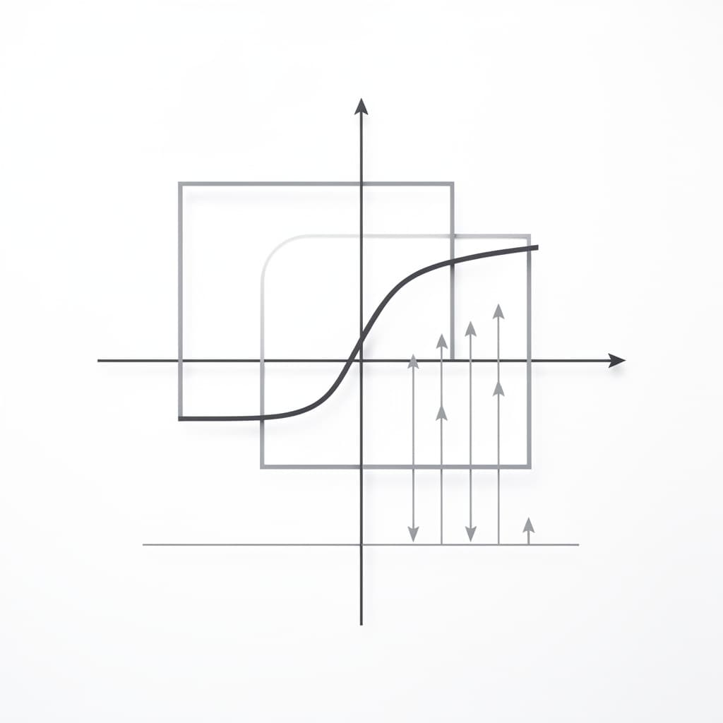
One of the most intuitive ways to grasp the concept is finding domain and range from a graph. To determine the domain visually, one looks at the horizontal extent of the graph along the $x$-axis. If you imagine a light shining from above and below the graph, the "shadow" cast on the $x$-axis represents the domain. Similarly, the range is the vertical extent of the graph along the $y$-axis, represented by the shadow cast if a light were shining from the left and right. If the graph of a function begins at $x = 1$ and continues indefinitely to the right, the domain is $[1, \infty)$. If the lowest point on the graph is at $y = -4$ and it extends upward forever, the range is $[-4, \infty)$.

Two essential diagnostic tools are the Vertical and Horizontal Line Tests. The Vertical Line Test is used to determine if a graph represents a function in the first place; if any vertical line intersects the graph at more than one point, the relation is not a function because it assigns multiple outputs to a single input. The Horizontal Line Test, while not used for the domain or range themselves, helps determine if a function is "one-to-one" (injective). If a horizontal line passes through multiple points, it indicates that different inputs produce the same output, which is a crucial realization when attempting to find the range of functions like $f(x) = x^2$ or $f(x) = \sin(x)$.

Visual analysis also reveals discontinuities and holes that algebraic formulas might hide at first glance. A "hole" (removable discontinuity) occurs when a factor is canceled out from the numerator and denominator of a rational function, such as $f(x) = (x-2)/(x-2)$. While the formula simplifies to $y = 1$, the original function is undefined at $x = 2$, creating a tiny gap in the line. On a graph, these are typically represented by an open circle. Vertical asymptotes, represented by dashed lines that the function approaches but never touches, indicate boundaries where the domain is restricted. Identifying these visual cues allows for a rapid and comprehensive assessment of a function's behavior without the immediate need for complex calculation.

6. Analytical Methods for Solving Boundaries

While graphs provide intuition, how to find domain and range algebraically requires a rigorous step-by-step approach. For the domain, the process involves setting up inequalities based on mathematical laws. If there is a square root, we set the expression inside the radical to be $\geq 0$ and solve for $x$. If there is a fraction, we set the denominator equal to zero to find the values that must be excluded. For instance, in the function $f(x) = \sqrt{2x - 6}$, we solve $2x - 6 \geq 0$, which yields $x \geq 3$. Thus, the domain is $[3, \infty)$. This algebraic method is foolproof and provides the exact boundaries that a visual inspection might only approximate.

Solving for the range algebraically is often more challenging and frequently involves inverse relations. If a function $f(x)$ is one-to-one, its range is the same as the domain of its inverse function, $f^{-1}(x)$. To find the range of $y = (2x+1)/(x-3)$, one can solve for $x$ in terms of $y$. By rearranging the equation, we get $x = (3y+1)/(y-2)$. Looking at this new expression, we can see that $y$ cannot be 2, because that would cause division by zero. Therefore, the range of the original function is all real numbers except 2. This "inverse domain" strategy is a powerful tool in a mathematician's arsenal, turning a difficult range problem into a standard domain problem.

Composite function dependencies introduce another layer of analytical complexity. When one function is nested inside another, such as $f(g(x))$, the domain of the composite function is restricted by both the domain of the inner function $g$ and the domain of the outer function $f$. Specifically, $x$ must be in the domain of $g$, and the resulting value $g(x)$ must be in the domain of $f$. For example, if $f(x) = \ln(x)$ and $g(x) = x - 5$, then for $f(g(x)) = \ln(x-5)$ to be defined, $x-5$ must be greater than zero. This chain of dependency ensures that every step of the transformation remains within the bounds of real-valued outputs, maintaining the integrity of the functional "pipeline."

7. Complex Structures and Transcendental Sets

The boundaries of logarithmic and exponential variations offer fascinating insights into the limits of growth and decay. Exponential functions of the form $f(x) = a \cdot b^x$ are defined for all real numbers $x$, but their range is strictly limited to $(0, \infty)$ (assuming $a > 0$). No matter how small or negative the exponent becomes, $b^x$ will never reach zero or become negative; it merely approaches the $x$-axis as a horizontal asymptote. Logarithmic functions are the inverses of exponentials, and their domains and ranges are swapped: the domain is $(0, \infty)$ and the range is $(-\infty, \infty)$. This symmetry highlights the deep connection between the two types of transcendental growth.

Trigonometric functions introduce periodic boundaries that repeat over specific intervals. The domain of $\sin(x)$ and $\cos(x)$ is all real numbers, but because of their circular nature, their range is confined to $[-1, 1]$. In contrast, functions like $\tan(x)$ and $\sec(x)$ have domains plagued by periodic vertical asymptotes. For example, $\sec(x) = 1/\cos(x)$ is undefined whenever $\cos(x) = 0$. Furthermore, the range of $\sec(x)$ is $(-\infty, -1] \cup [1, \infty)$, meaning there is a "gap" in the output between -1 and 1. These periodic restrictions are essential in fields like acoustics and electrical engineering, where wave functions must be carefully bounded to avoid signal distortion.

The domain of a function is the set of all possible input values (independent variable) which produce a valid output, while the range is the set of all possible output values (dependent variable) that result from those inputs.

Piecewise function domain integration requires a segmented approach to boundary analysis. A piecewise function is defined by different formulas over different intervals of its domain. To find the total domain, one must take the union of all the individual intervals specified in the function's definition. The range, however, is the union of the ranges of each individual "piece" across its specified interval. For example, if a function is defined as $f(x) = x^2$ for $x < 0$ and $f(x) = x + 1$ for $x \geq 0$, the range would be the combination of $(0, \infty)$ from the first part and $[1, \infty)$ from the second, resulting in $(0, \infty)$. Mapping piecewise boundaries requires meticulous attention to the endpoints and the behavior of each distinct branch.

8. Synthesizing Domain and Range Examples

To truly master the subject, one must analyze how transformations affect the domain and range examples seen in common curricula. Take the quadratic function $f(x) = a(x - h)^2 + k$. The domain remains $(-\infty, \infty)$, but the range is determined by the vertex $(h, k)$ and the leading coefficient $a$. If $a$ is positive, the parabola opens upward, and the range is $[k, \infty)$. If $a$ is negative, it opens downward, and the range is $(-\infty, k]$. This synthesis shows that the range is not a static property of "quadratics" but a dynamic result of the function's specific transformations and orientation in space.

Absolute value and step functions provide additional case studies in boundary mapping. The absolute value function $f(x) = |x|$ has a domain of all real numbers and a range of $[0, \infty)$, similar to $x^2$. However, its transformations, such as $f(x) = -|x + 2| + 5$, shift the range to $(-\infty, 5]$. Step functions, such as the greatest integer function $f(x) = \lfloor x \rfloor$, have a domain of all real numbers, but their range is a discrete set of integers $\{\dots, -2, -1, 0, 1, 2, \dots\}$. These examples demonstrate that the range does not always have to be a continuous interval; it can be a "ladder" of individual points, depending on the logic of the function's mapping.

Finally, rational functions with complex vertical asymptotes and slant asymptotes challenge our ability to find boundaries analytically. Consider a function where the degree of the numerator is exactly one higher than the degree of the denominator, such as $f(x) = (x^2 + 1)/(x - 1)$. This function will have a vertical asymptote at $x = 1$ (restricting the domain) and a slant asymptote, which influences the range as $x$ approaches infinity. By performing long division, we can see the function's end behavior more clearly. Such advanced examples synthesize all the skills discussed: algebraic restriction, visual asymptotic analysis, and interval notation, providing a complete picture of how we map the mathematical boundaries of the world around us.

References

- Stewart, J., "Calculus: Early Transcendentals, 8th Edition", Cengage Learning, 2015.
- Larson, R., & Edwards, B. H., "Precalculus", Cengage Learning, 2017.
- Spivak, M., "Calculus", Publish or Perish, 2008.
- Abramson, J. P., "Algebra and Trigonometry", OpenStax, 2015.
Recommended Readings
- The Pleasures of Counting by T.W. Körner — A brilliant look at how mathematical functions and their boundaries apply to real-world history and problem-solving.
- A Tour of the Calculus by David Berlinski — An engaging, narrative-driven exploration of the foundational concepts of functions, limits, and the continuity of the real line.
- Infinite Powers by Steven Strogatz — This book explains how calculus, built upon functional relationships, has shaped the modern world, making abstract boundaries feel tangible.