The Structural Logic of Graph Traversal

The fundamental challenge of computer science lies not merely in storing data, but in efficiently navigating the complex relationships between discrete entities. Graph traversal algorithms serve as the primary mechanism for this navigation, providing a systematic way to visit every node within a network structure. Whether exploring a social network, mapping the internet, or solving a puzzle, the underlying logic remains consistent: we must track which nodes have been discovered, which are currently being explored, and which remain hidden in the darkness of the unknown. The choice of strategy—deciding whether to prioritize width or depth—fundamentally alters the algorithm's performance, memory consumption, and suitability for specific problem domains. Understanding the nuances of bfs vs dfs is therefore essential for any practitioner seeking to optimize computational workflows.

The Mechanics of Exploration

In the realm of discrete mathematics, a graph is defined as a collection of vertices connected by edges. The structural logic of graph traversal begins with the concept of adjacency, where two nodes are considered neighbors if an edge exists between them. Connectivity determines the reachability of these nodes; a graph is connected if there is a path between every pair of vertices. When an algorithm begins its execution, it must maintain a record of visited nodes to avoid infinite loops, particularly in graphs containing cycles. This record-keeping is the cornerstone of traversal, transforming a chaotic web of connections into a structured sequence of discoveries.

The concept of graph traversal algorithms centers on the "frontier"—the boundary between the explored and unexplored regions of the graph. As the algorithm progresses, it expands this frontier by selecting an active node and examining all of its adjacent neighbors. This process continues until the frontier is empty, meaning all reachable nodes have been processed. While all traversal algorithms share the goal of visiting vertices, they differ significantly in their search frontier management. By changing the data structure used to store the frontier, we fundamentally change the order of discovery, leading us to the two primary methodologies: Breadth First Search and Depth First Search.

Breadth First Search: The Layered Approach

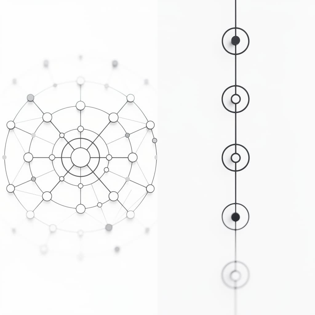
Breadth First Search (BFS) operates on a principle of radial expansion, much like ripples moving outward from a stone dropped in a pond. It explores the graph in a level-order discovery pattern, ensuring that all nodes at a distance $k$ from the starting source are visited before any nodes at distance $k+1$ are considered. This exhaustive lateral movement makes BFS particularly powerful for finding the shortest path in unweighted graphs, as it guarantees that the first time a target node is encountered, the path taken to reach it is the shortest possible. The algorithm essentially layers the graph into concentric circles of increasing distance from the origin.

The execution model of BFS relies heavily on a queue-based architecture, following a First-In, First-Out (FIFO) logic. When a node is visited, its neighbors are added to the back of the queue, while the node currently at the front is removed and processed. This ensures that the oldest discovered nodes—those closest to the start—are always prioritized over newly discovered ones. By maintaining this strict ordering, BFS avoids the risk of wandering deep into one branch of the graph while leaving nearby nodes unvisited. This systematic progression requires more memory to store the frontier in wide graphs, but it provides a predictable and stable discovery path that is vital for network broadcasting and peer-to-peer discovery.

from collections import deque

def breadth_first_search(graph, start_node):
    visited = {start_node}
    queue = deque([start_node])
    
    while queue:
        current = queue.popleft()
        print(f"Visited: {current}")
        
        for neighbor in graph[current]:
            if neighbor not in visited:
                visited.add(neighbor)
                queue.append(neighbor)

Depth First Search: The Path of Recursion

In contrast to the radial expansion of BFS, Depth First Search (DFS) follows a strategy of exhaustive exploration along a single path. It behaves like a navigator in a maze who chooses a direction and follows it as far as possible until a dead end or a previously visited node is reached. Only when it can go no further does the algorithm backtrack to the most recent decision point to try a different branch. This "deep dive" approach allows DFS to reach the far corners of a graph quickly, making it highly effective for problems involving connectivity, cycle detection, and topological sorting in directed acyclic graphs.

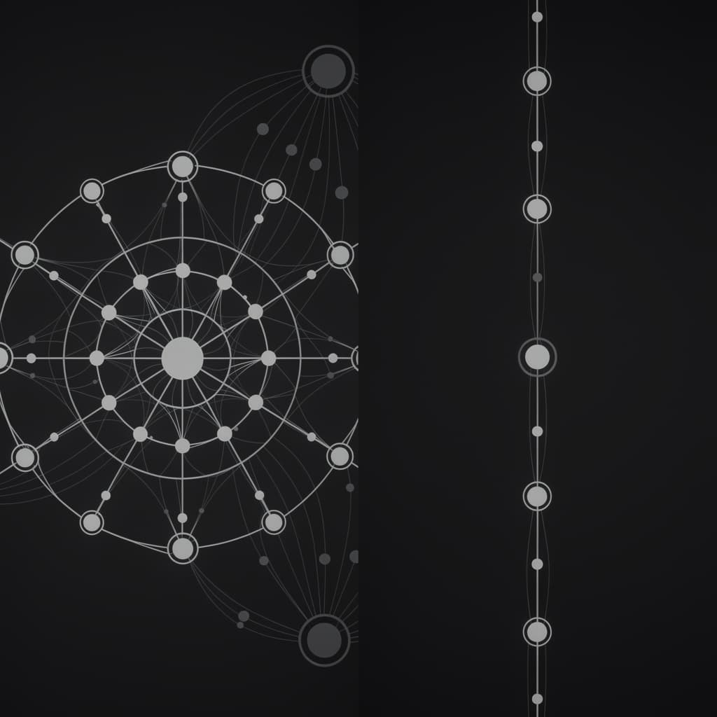
The structural logic of DFS is fundamentally stack-based, utilizing a Last-In, First-Out (LIFO) mechanism. While this can be implemented with an explicit stack data structure, it is most commonly achieved through recursion, where the system's call stack manages the state of the traversal. Each recursive call represents a step deeper into the graph; when a function returns, the algorithm naturally backtracks to the previous vertex. Because DFS only needs to keep track of the current path from the source to the leaf, it often uses significantly less memory than BFS when navigating graphs with high branching factors but moderate depth.

def depth_first_search(graph, current_node, visited=None):
    if visited is None:
        visited = set()
    
    visited.add(current_node)
    print(f"Visited: {current_node}")
    
    for neighbor in graph[current_node]:
        if neighbor not in visited:
            depth_first_search(graph, neighbor, visited)

Architectural Divergence: BFS and DFS Differences

The primary architectural difference between bfs and dfs lies in the shape of the search frontier and the resulting memory utilization. In a wide graph with a large branching factor, BFS must store all nodes at the current level in its queue, which can lead to a space complexity that grows linearly with the width of the graph. Conversely, DFS only stores the nodes on the current path, meaning its memory usage is proportional to the maximum depth of the graph. If a graph represents a state space that is incredibly deep or infinite, DFS might struggle or fail to terminate without depth-limiting, whereas BFS might exhaust available RAM if the search space is too wide.

Another divergence is found in how these algorithms handle the search frontier management. BFS treats all neighbors with equal priority relative to their distance from the start, creating a "uniform" expansion. DFS, however, exhibits a "greedy" behavior toward depth, prioritizing the most recently discovered neighbor. This leads to different traversal orders even on the same graph: BFS might visit nodes in the order $A,B,C,D$, while DFS might visit them as $A,B,D,C$. These differences are not merely academic; they dictate which algorithm is appropriate for real-time applications, such as AI in gaming, where a DFS-based approach might allow a character to explore a specific room fully before moving to the next, while BFS would force the character to check every doorway in a hallway before entering any of them.

Computational Efficiency and Performance

When analyzing the time complexity of bfs and dfs, both algorithms are remarkably efficient, typically operating in $O(V+E)$ time, where $V$ represents the number of vertices and $E$ represents the number of edges. This linear time complexity assumes that the graph is represented using an adjacency list, allowing for constant-time access to a node's neighbors. In practice, this means that the time taken to traverse the graph scales directly with the size of the data structure. Whether you choose BFS or DFS, the algorithm will visit each node and edge exactly once, provided a "visited" set is maintained to prevent redundant processing.

Despite identical time complexities, the auxiliary space requirements differ based on the graph's topology. In a perfectly balanced binary tree of depth $H$, BFS would require $O(2^H)$ space to store the leaf nodes in the queue, while DFS would only require $O(H)$ space for the recursion stack. However, in a skewed graph that resembles a linked list, DFS would require $O(V)$ space for the stack, while BFS would only require $O(1)$ for the queue. Therefore, the choice of "bfs vs dfs" should be informed by the expected "shape" of the data, as shown in the following comparison table:

Feature	Breadth First Search (BFS)	Depth First Search (DFS)
Data Structure	Queue (FIFO)	Stack (LIFO) or Recursion
Discovery Order	Level-by-level (horizontal)	Path-by-path (vertical)
Space Complexity	$O(W)$ where $W$ is max width	$O(D)$ where $D$ is max depth
Shortest Path	Optimal for unweighted graphs	Not guaranteed to find shortest path
Best Case Use	Target is near the source	Target is far from the source

Strategic Implementation and Practical Use Cases

Determining when to use bfs vs dfs is a critical skill in algorithmic design. BFS is the undisputed choice when the goal is to find the shortest path in unweighted graphs. For instance, in social networking applications, finding the "degrees of separation" between two users is a BFS problem because we want the minimum number of connections. Similarly, in GPS navigation systems calculating routes based on the fewest number of turns, BFS ensures that we explore all immediate options before venturing further away, guaranteeing optimality in the number of edges traversed.

On the other hand, DFS excels in scenarios requiring exhaustive exploration or structural analysis. It is the backbone of algorithms for topological sorting, which is used in task scheduling and build systems (like Make or Gradle) to determine the correct order of operations based on dependencies. DFS is also preferred for solving puzzles like Sudoku or mazes, where the algorithm must commit to a path, evaluate its success, and backtrack if necessary. Because DFS naturally explores entire branches, it is also used in web crawlers that need to explore the deep hierarchy of a specific domain before moving to external links.

Topological Constraints and Specialized Structures

Beyond simple pathfinding, graph traversal is used to identify complex topological properties. Detecting cycles is one of the most common applications; in an undirected graph, both algorithms can detect cycles by identifying an edge that points back to a previously visited node that is not the immediate parent. However, in directed graphs, DFS is uniquely suited for this task through the identification of "back edges"—edges that point to an ancestor in the current recursion stack. This is vital in compiler design to detect circular dependencies in module imports or variable definitions.

Furthermore, BFS is frequently employed to check for bipartite matching and connectivity. A graph is bipartite if its vertices can be divided into two independent sets such that every edge connects a vertex in one set to a vertex in the other. By using BFS to "color" nodes with alternating colors level by level, we can easily detect a conflict; if two adjacent nodes are assigned the same color, the graph is not bipartite. DFS, conversely, is the preferred method for finding strongly connected components in directed graphs using algorithms like Kosaraju's or Tarjan's, which rely on the post-order traversal properties inherent to the depth-first approach.

Algorithmic Evolution in Modern Systems

As we transition into the era of Big Data, the logic of traversal has evolved to handle large-scale networks that exceed the memory of a single machine. In distributed systems like Apache Spark or GraphX, traversal is often parallelized. Distributed BFS, for example, involves "frontier expansion" across multiple nodes in a cluster, where each machine processes its local vertices and communicates the discovery of new neighbors to other machines via message passing. This allows for the traversal of trillion-edge graphs, such as the global web graph or massive financial transaction networks, where traditional single-threaded BFS would be impractical.

Modern implementations also incorporate heuristic enhancements to guide the search process. While pure BFS and DFS are uninformed—meaning they have no knowledge of where the goal might be—algorithms like A* (A-Star) combine the level-order logic of BFS with a heuristic function to prioritize paths that look more promising. This optimization is crucial in artificial intelligence and robotics, where an agent must navigate a physical space efficiently. By blending the exhaustive nature of classical traversal with predictive mathematical models, developers can create systems that navigate complex environments with human-like intuition and mathematical precision.

References

- Cormen, T. H., Leiserson, C. E., Rivest, R. L., & Stein, C., "Introduction to Algorithms", MIT Press, 2022.
- Sedgewick, R., & Wayne, K., "Algorithms, 4th Edition", Addison-Wesley Professional, 2011.
- Kleinberg, J., & Tardos, É., "Algorithm Design", Pearson, 2005.
- Russell, S., & Norvig, P., "Artificial Intelligence: A Modern Approach", Pearson, 2020.
Recommended Readings
- The Art of Computer Programming, Volume 1: Fundamental Algorithms by Donald Knuth — A foundational text that provides the mathematical rigorousness behind the data structures used in traversal.
- Graph Algorithms by Shimon Even — A deep dive into the theoretical aspects of graph theory and the proofs of correctness for BFS and DFS.
- Networks, Crowds, and Markets by Easley and Kleinberg — An excellent resource for understanding how these algorithms are applied to real-world social and economic networks.
Turn this topic into a full course
Noesis builds the syllabus, notes and tests for you, and you study them with a tutor that knows your material.